Package demo for scRNAseqApp
Jianhong Ou1
Source:vignettes/workshop_scRNAseqApp.Rmd
workshop_scRNAseqApp.RmdIntroduction
Single-cell RNA sequencing (scRNA-seq) is a powerful technique to study gene expression, cellular heterogeneity, and cell states within samples in single-cell level. The development of scRNA-seq shed light to address the knowledge gap about the cell types, cell interactions, and key genes involved in biological process and their dynamics. To precisely meet the publishing requirement, reduce the time of communication the bioinformatician with researchers, and increase the re-usability and reproducibility of scientific findings, multiple interactive visualization tools, such as Loupe Browser1 and cellxgene2, were developed to provide the researchers access to the details of the data. In R/Bioconductor, there are options to use the flexibility of the R-graphics system to display the status of single-cell.
Table 1: R/Bioconductor available tools for interactive scRNA-Seq data visualization.
| software | description |
|---|---|
| Asc-Seurat3 | Asc-Seurat, also known as Analytical single-cell Seurat-based web application, is a user-friendly web application built on the Shiny framework. Its name, pronounced as “ask Seurat,” reflects its purpose of simplifying scRNA-seq analysis. With a click-based interface and straightforward installation process, Asc-Seurat enables users to effortlessly execute all essential steps for scRNA-seq analysis. Moreover, it seamlessly incorporates the powerful features of Seurat and Dynverse, providing users with a comprehensive toolkit. Additionally, Asc-Seurat offers the convenient functionality of instant gene functional annotation using BioMart. |
| BingleSeq4 | BingleSeq was created as an intuitive application to offer a user-friendly solution for analyzing count matrices from both Bulk and Single-cell RNA-Seq experiments. BingleSeq goes beyond basic functionality and includes additional features like visualization techniques, comprehensive functional annotation analysis, and rank-based consensus for differential gene analysis results. |
| CellView5 | CellView is designed to efficiently extract expression, dimensionality reduction/clustering, and feature annotation data objects from an .Rds file. It offers 3D visualization, (co-)expression pattern plots, and on-the-fly differential gene expression analysis. |
| ChromSCape6 | ChromSCape, an application designed for Single Cells Chromatin landscape profiling, offers a user-friendly and readily deployable Shiny Application. It is specifically tailored for the analysis of various single-cell epigenomics datasets such as scChIP-seq, scATAC-seq, scCUT&Tag, and more. ChromSCape provides a seamless workflow, starting from aligned data to differential analysis and gene set enrichment analysis. |
| Granatum7 | Granatum: a web-based scRNA-Seq analysis pipeline designed for accessible research. With a user-friendly graphical interface, users can navigate the pipeline effortlessly, adjusting parameters and visualizing results. Granatum guides users through diverse scRNA-Seq analysis steps, encompassing plate merging, batch-effect removal, outlier-sample removal, normalization, imputation, gene filtering, cell clustering, differential gene expression analysis, pathway/ontology enrichment analysis, protein network interaction visualization, and pseudo-time cell series construction. |
| InterCellar8 | InterCellar empowers researchers to conduct interactive analysis of cell-cell communication results derived from scRNA-seq data. By utilizing pre-computed ligand-receptor interactions, InterCellar offers filtering options, annotations, and various visualizations to explore clusters, genes, and functions. Additionally, InterCellar leverages functional annotation from Gene Ontology and pathway databases, enabling data-driven analyses to investigate cell-cell communication in one or multiple conditions. |
| iS-CellR9 | iS-CellR, an Interactive platform for Single-cell RNAseq, is a web-based Shiny application that offers a comprehensive analysis of single-cell RNA sequencing data. It provides a rapid approach for filtering and normalizing raw data, performing dimensionality reductions (both linear and non-linear) to identify cell type clusters, conducting differential gene expression analysis to pinpoint markers, and exploring inter-/intra-sample heterogeneity. iS-CellR seamlessly integrates the Seurat package with Shiny’s reactive programming framework and employs interactive visualization using the plotly library. |
| iSEE10 | iSEE is a package that offers an interactive user interface for data exploration within objects derived from the SummarizedExperiment class. It specifically caters to single-cell data stored in the SingleCellExperiment derived class. The user interface is built using RStudio’s Shiny framework and features a multi-panel layout for effortless navigation. iSEE is the winners of the 1st Shiny Contest |
| PIVOT11 | PIVOT offers comprehensive support for routine RNA-Seq data analysis. It includes essential functionalities such as normalization, differential expression analysis, dimension reduction, correlation analysis, clustering, and classification. With PIVOT, users can effortlessly complete workflows utilizing DESeq2, monocle, and scde packages with just a few clicks. Additionally, all analysis reports can be easily exported, and the program state can be saved, loaded, and shared for seamless collaboration. |
| SC112 | SC1 offers an integrated workflow for scRNA-Seq analysis, introducing a novel approach to selecting informative genes using term-frequency inverse-document-frequency (TF-IDF) scores. It encompasses various methods for clustering, differential expression analysis, gene enrichment, interactive visualization, and cell cycle analysis. Furthermore, the tool seamlessly integrates additional single-cell omics data modalities, such as T-cell receptor (TCR)-Seq, and supports multiple single-cell sequencing technologies. With its streamlined process, researchers can swiftly generate a comprehensive analysis and derive valuable insights from their scRNA-Seq data. |
| SCANNER13 | SCANNER utilizes Seurat object, created through the Seurat pipeline, as its input. It leverages the Seurat 3.0 package to conduct various data analyses, including data normalization, high variable feature selection, data scaling, dimension reduction, and cluster identification. |
| scClustViz14 | scClustViz is a user-friendly R Shiny tool to visualize clustering results from common single-cell RNAseq analysis pipelines. The tool serves two primary purposes: A) assisting in the selection of a biologically relevant resolution or K from clustering results by assessing differential expression between the resulting clusters, and B) facilitating cell type annotation and identification of marker genes. |
| scSVA15 | scSVA (single-cell Scalable Visualization and Analytics) is a highly optimized tool designed for efficient visualization of cells on 2D or 3D embeddings. It specializes in extracting cell features for visualization from compressed big expression matrices stored in HDF5, Loom, and text file formats. Utilizing VaeX as a powerful Python library for grid-based vector data processing and integrating Shiny for its user interface, scSVA delivers high-performance analytics. The tool enables basic statistical analysis, such as computing cell counts and distributions of gene expression values across selected or provided cell groups. Moreover, users can leverage scSVAtools to interactively run fast methods for diffusion maps and 3D force-directed layout embedding (FLE), further enhancing their analysis capabilities. |
| SeuratV3Wizard16/NASQAR | NASQAR (Nucleic Acid SeQuence Analysis Resource) offers a user-friendly interface that enables users to conveniently and effectively explore their data interactively. It supports popular tools for diverse applications, including Transcriptome Data Preprocessing, RNAseq Analysis (including Single-cell RNAseq), Metagenomics, and Gene Enrichment. |
| ShinyArchRUiO17 | ShinyArchR.UiO, short for ShinyArchR User interface Open, provides an integrative environment for visualizing large-scale single-cell chromatin accessibility data (scATAC-seq). Built upon ArchR18, ShinyArchR.UiO offers a seamless and interactive experience for exploring and analyzing scATAC-seq datasets. |
| ShinyCell19 | ShinyCell is an R package that empowers users to develop interactive web applications based on Shiny for visualizing single-cell data. It offers a range of visualization options, including the ability to visualize cell information and gene expression on reduced dimensions like UMAP. Users can also explore the coexpression of two genes on reduced dimensions and visualize the distribution of continuous cell information, such as nUMI or module scores, using violin plots or box plots. ShinyCell further allows users to visualize the composition of different clusters or groups of cells using proportion plots and examine the expression of multiple genes using bubble plots or heatmaps. |
| singleCellTK20 | The singleCellTK R package provides the Single Cell Toolkit (SCTK) facilitates the importation of raw or filtered counts from various scRNAseq preprocessing tools like 10x CellRanger, BUStools, Optimus, STARSolo, and more. It incorporates publicly available R or Python tools to enable comprehensive quality control, including doublet detection and ambient RNA removal. SCTK integrates analysis workflows from popular tools such as Seurat and Bioconductor/OSCA into a unified framework, allowing users to perform diverse analyses. The results from these workflows can be summarized and shared conveniently using comprehensive HTML reports. Additionally, data can be exported to Seurat or AnnData object formats, enabling seamless integration with other downstream analysis workflows. |
Based on ShinyCell, the scRNAseqApp package is developed with multiple highly interactive visualizations of how cells and subsets of cells cluster behavior for scRNA-seq, scATAC-seq and sc-multiomics data. The scRNAseqApp is designed to efficiently extract expression, dimensional reduction/clustering, and feature annotation data objects in multiple interactive manners with highly customized filter conditions by selecting metadata. It offers a user-friendly interface that facilitates the exploration and interactive analysis of single-cell transcriptomic, and multiomic data.
Key features of scRNAseqApp include:
(Co-)Expression Patterns: Users can delve into expression patterns within specific clusters or among clusters, enabling a detailed examination of gene co-expression. It provides a three-dimensional visualization of the co-expression data, enhancing the understanding of the relationships between genes.
Side-by-Side Data Visualization: The scRNAseqApp allows for the simultaneous visualization of transcriptomic or multiomic data. Users can easily compare expression patterns, cell metadata, or chromatin accessibility across different subsets of cells, facilitating comprehensive data exploration.
All-in-One Page Visualization: With the scRNAseqApp, users can visualize up to eight different types of figures on a single page. This consolidated view provides a comprehensive overview of the data, enhancing data interpretation and analysis.
Search Tool for Datasets: The scRNAseqApp includes a convenient search tool that enables users to search for specific expression patterns across all available datasets. The search results are presented as informative waffle plots, simplifying the identification and comparison of expression patterns.
User Management System: To ensure data security and protect unpublished data, the scRNAseqApp incorporates a user management system. This system controls access and permissions, allowing researchers to safeguard their valuable datasets.
The scRNAseqApp combines these features to provide a comprehensive and user-friendly platform for the analysis and exploration of single-cell transcriptomic and multiomic data, empowering researchers in their investigations.
Installation
BiocManager is used to install the released version of scRNAseqApp.
library(BiocManager)
install("scRNAseqApp")
To check the current version of scRNAseqApp, please try
packageVersion("scRNAseqApp")
#> [1] '1.1.9'
Quick guide for scRNAseqApp with a subset of PBMC21 scRNA-Seq data
The package includes a subset of PBMC sample data. To demonstrate the package, there are three simple and straightforward steps.
Step 3. Start shiny APP
scRNAseqApp(app_path = publish_folder)Shiny pages
The homepage showcases a streamlined search bar with a minimalist design. Conducting a keyword search will generate a list of results with hyperlinks, while searching by gene symbols will display waffle plots for each dataset. The waffle plots demonstrate the proportion of cell numbers compared to the largest cell group and use a heatmap to indicate expression levels. These waffle plots are also accessible in the ‘stats’ module, offering an interactive mode.
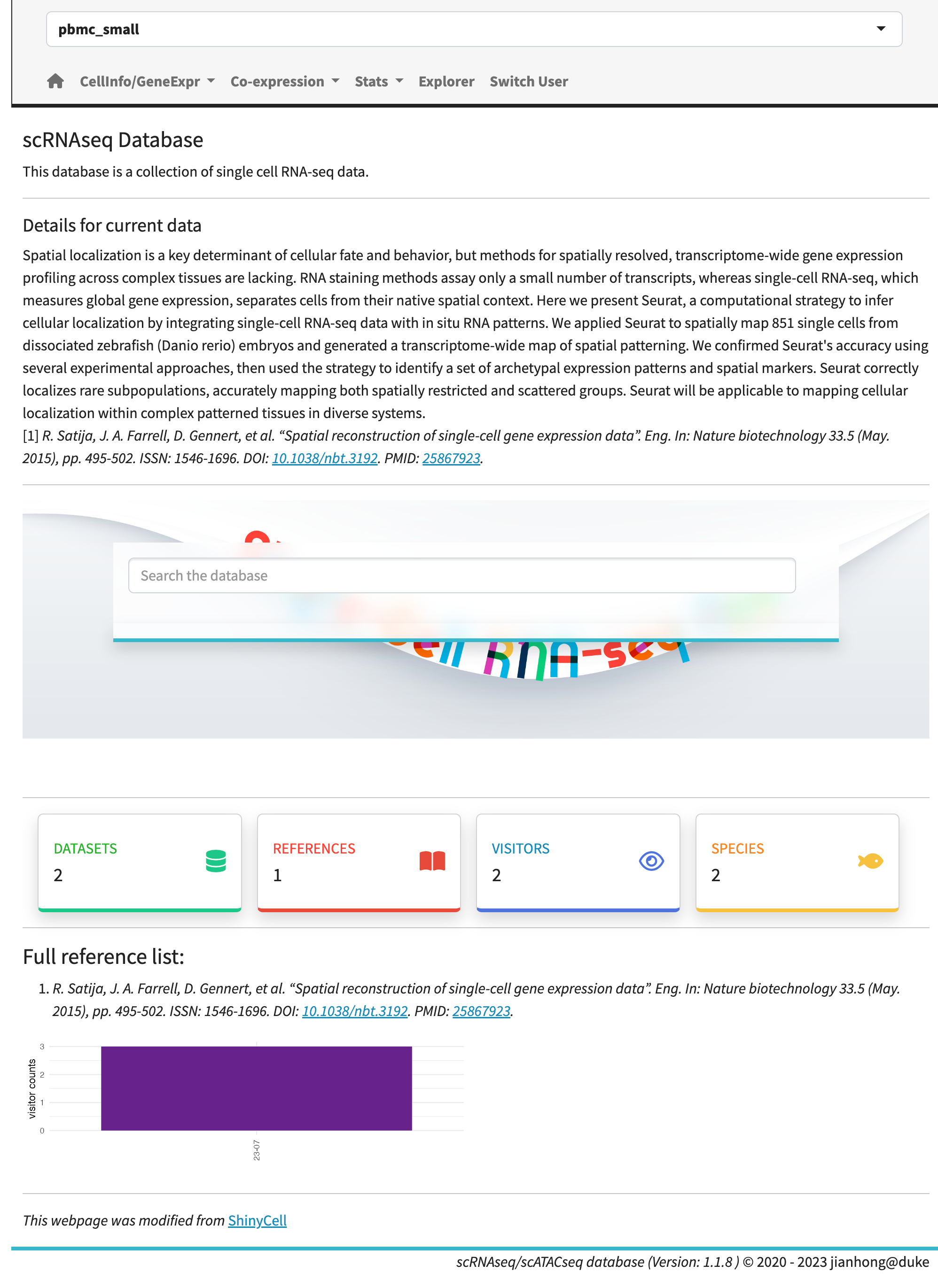
Home page.
To facilitate data visualization, we have developed four primary modules:
- side-by-side plots of cell information and gene expression,
- co-expression plots,
- statistical plots,
- and an explorer for multiple combination plots.
Each module comprises a main panel and a plot panel. In the main panel, users can subset cells and control plot parameters, while the plot panel is used to visualize the data, present statistical tables, and offer a download button.
Here is a short video for the web pages:
Side-by-side plots of cell information and gene expression
The exploration of expression profiles side by side is facilitated through four sub-modules:
- cell information vs. gene expression,
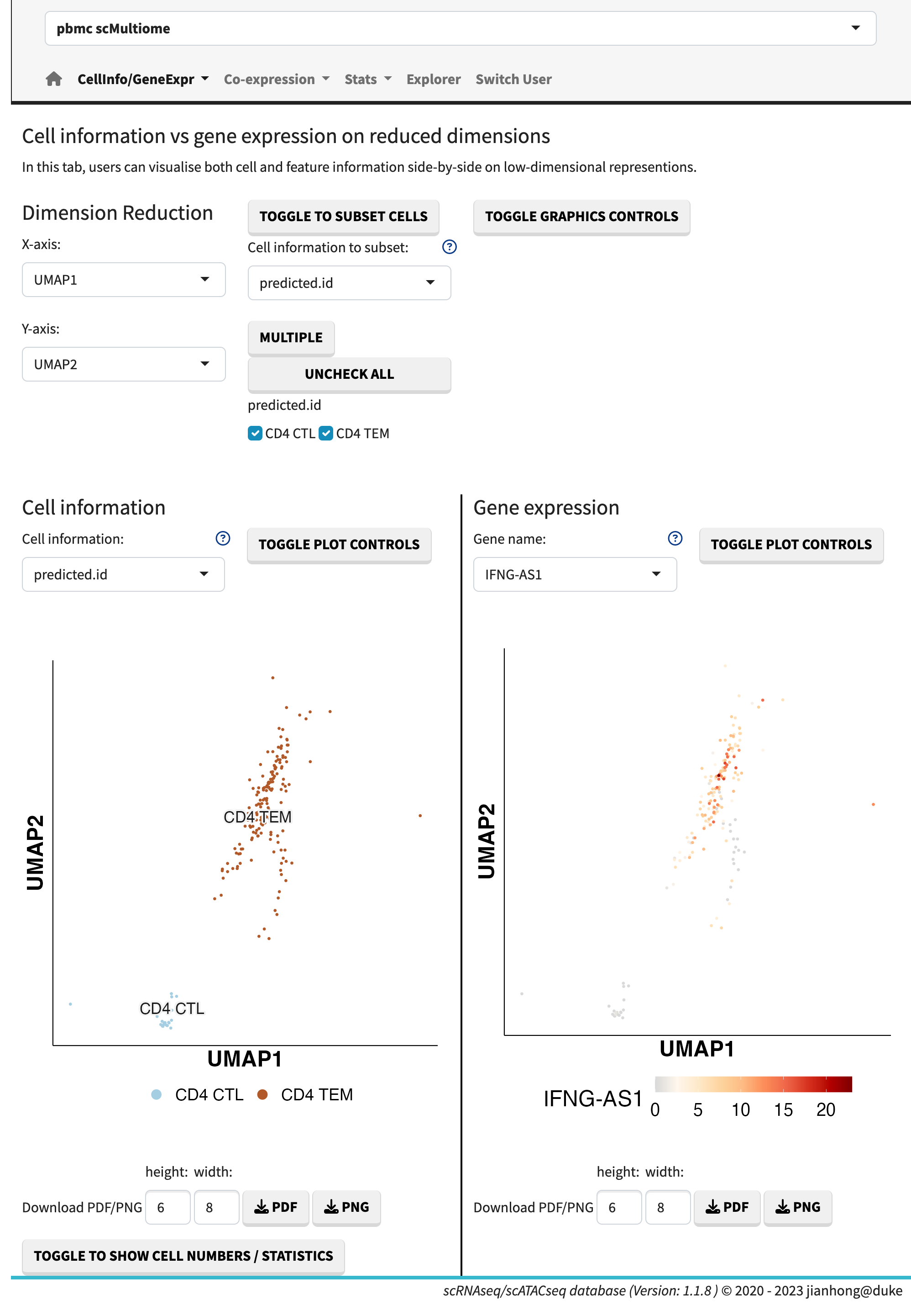
Cell information vs. gene expression
- cell information vs. cell information,
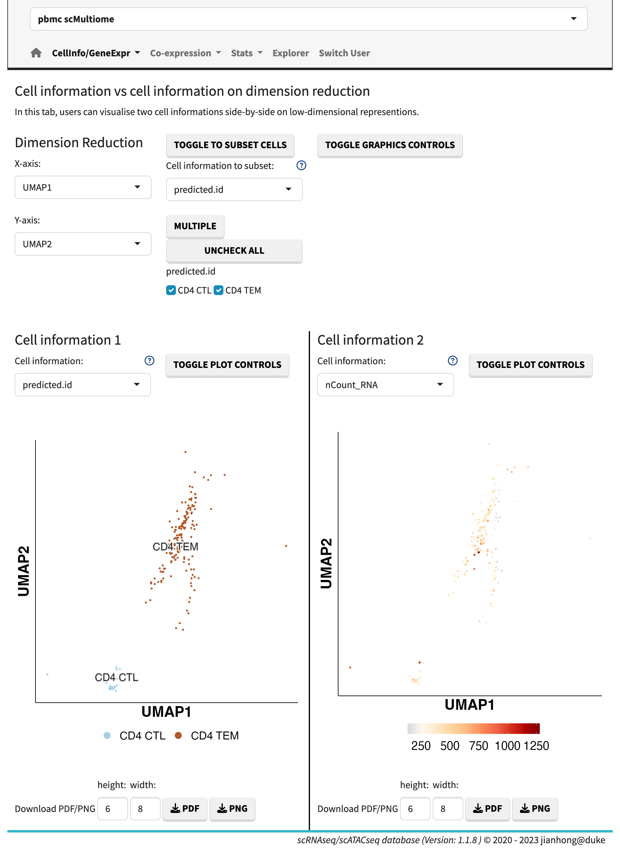
Cell information vs. cell information
- gene expression for different subsets of cells,
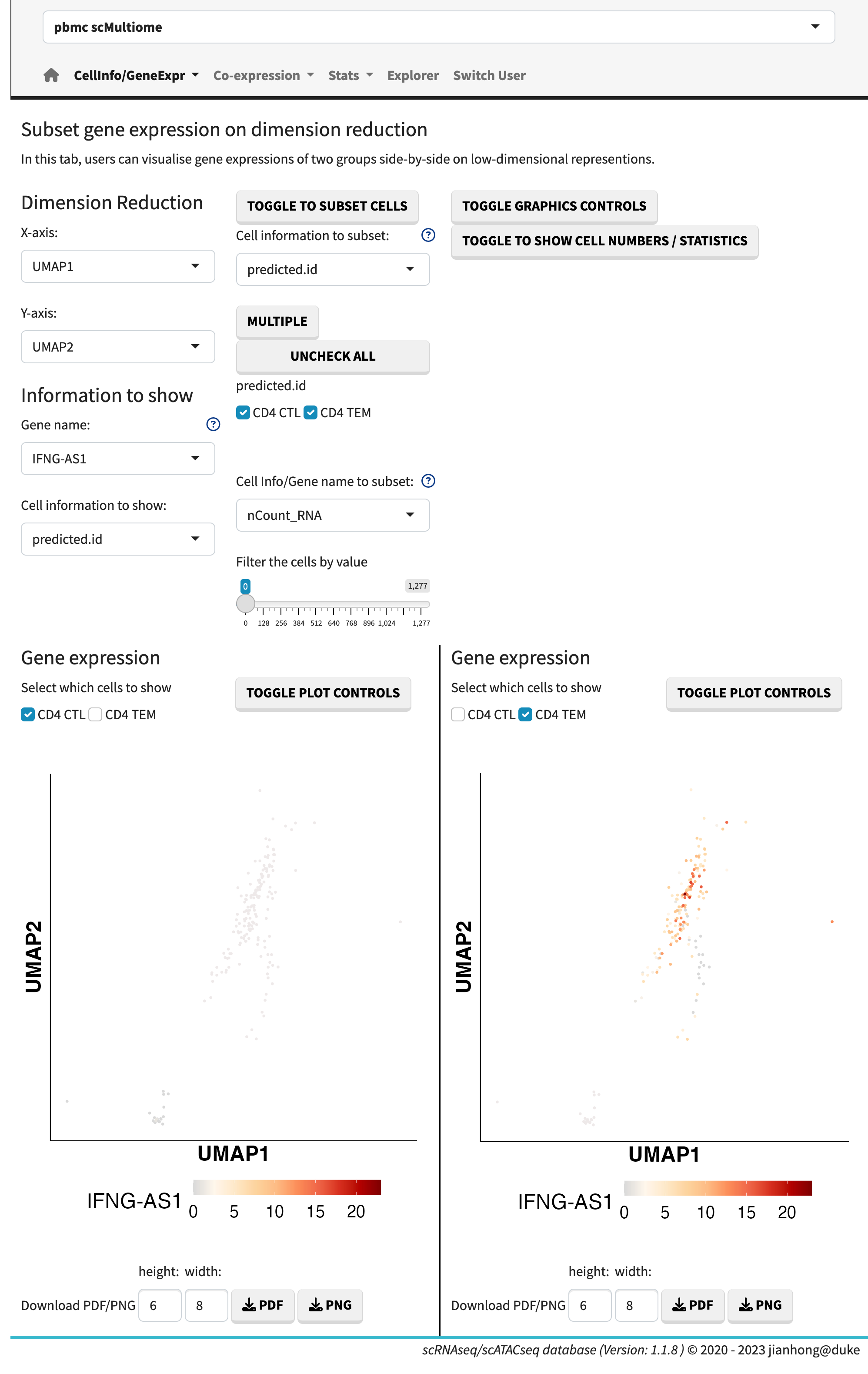
Subset gene expression
- and gene accessibility vs. gene expression.
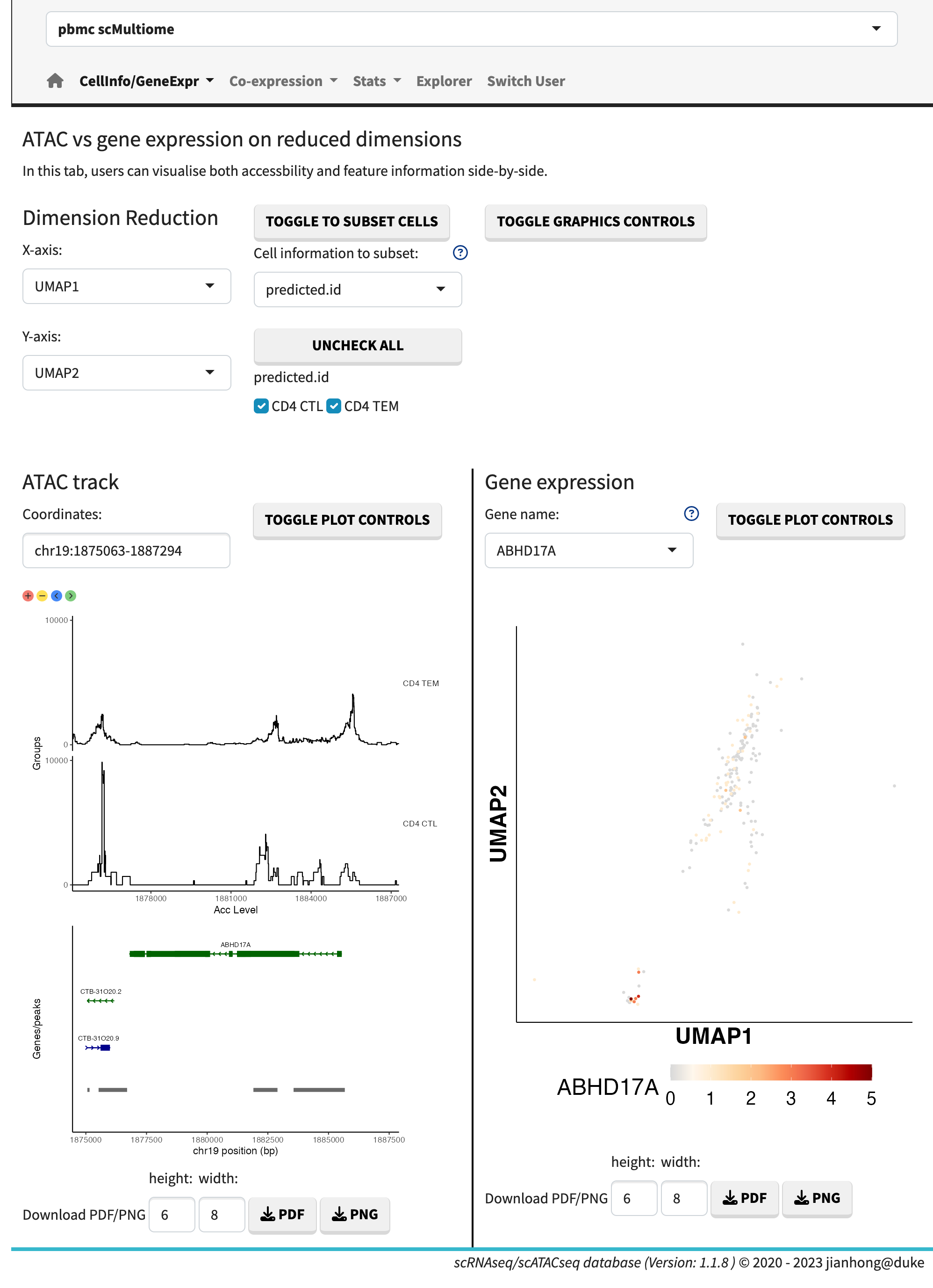
Multiome plots
The cell information refers to the metadata associated with each cell. The gene expression data can be visualized using dots plots (default) or ridge plots by adjusting the plot controls. Users have the flexibility to manually set the maximum expression value, enabling the comparison of plots across different genes.
Co-expression plots
To explore the co-expression of two or several genes, there are four sub-modules available:
- gene expression vs. gene expression,
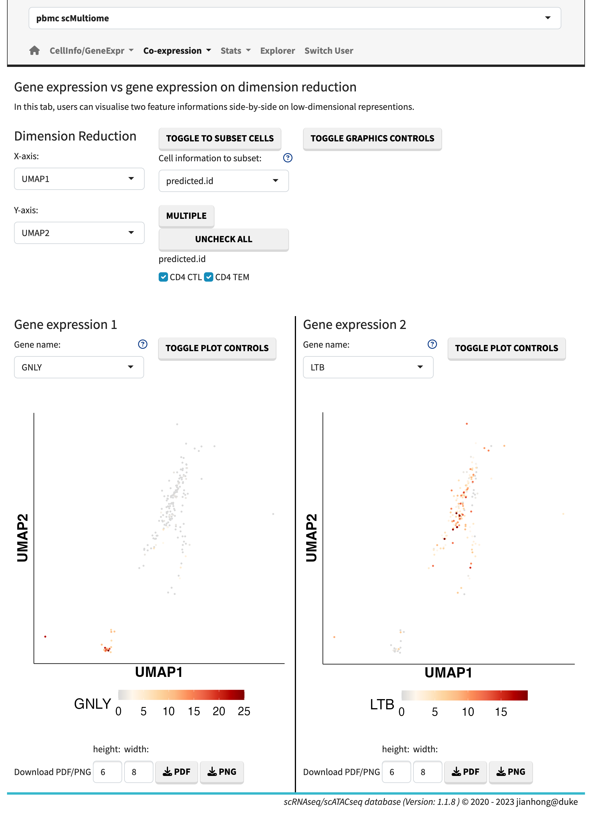
Gene expression vs. expression
- gene co-expression plot,
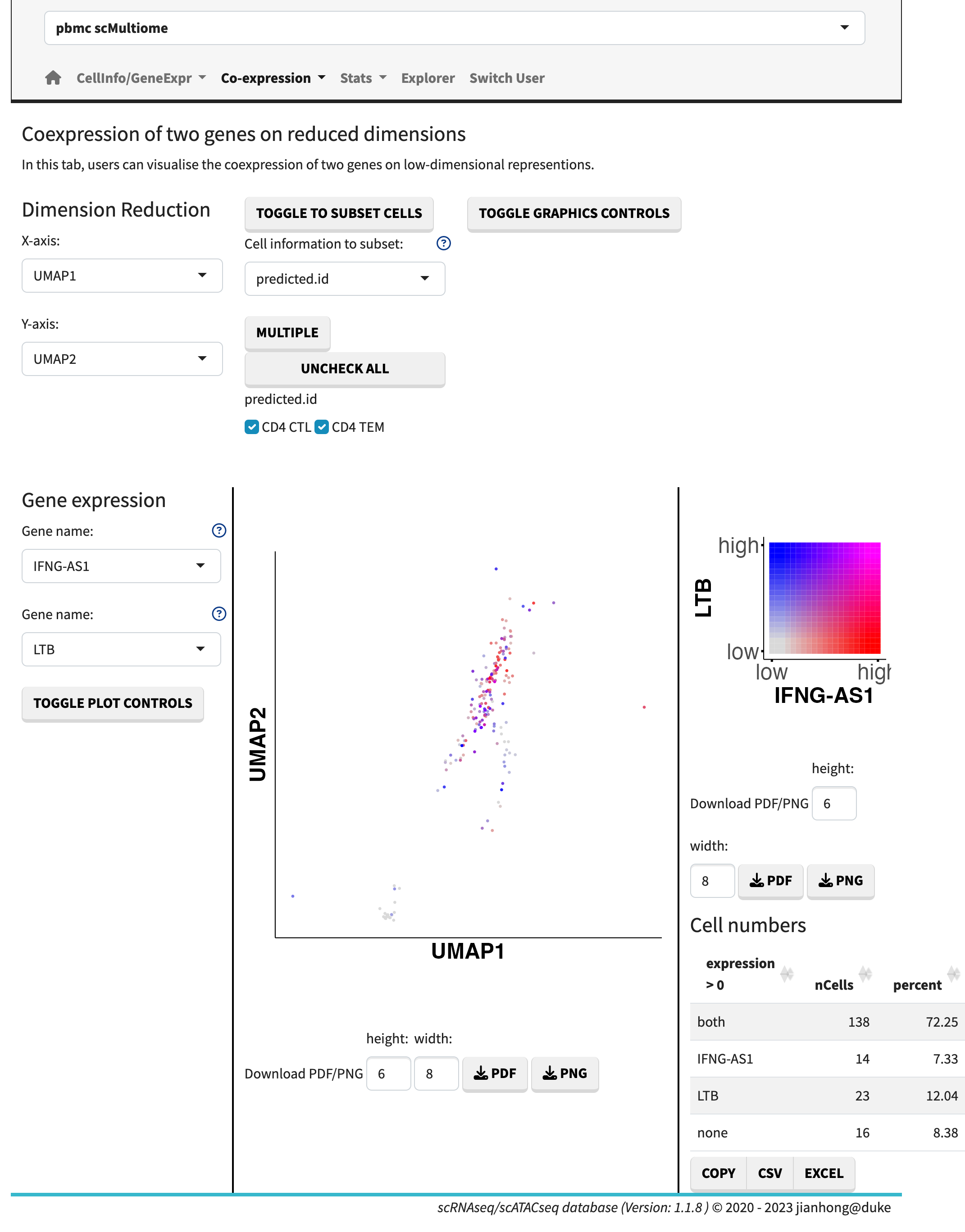
Co-expression
- 3-dim gene co-expression plot,
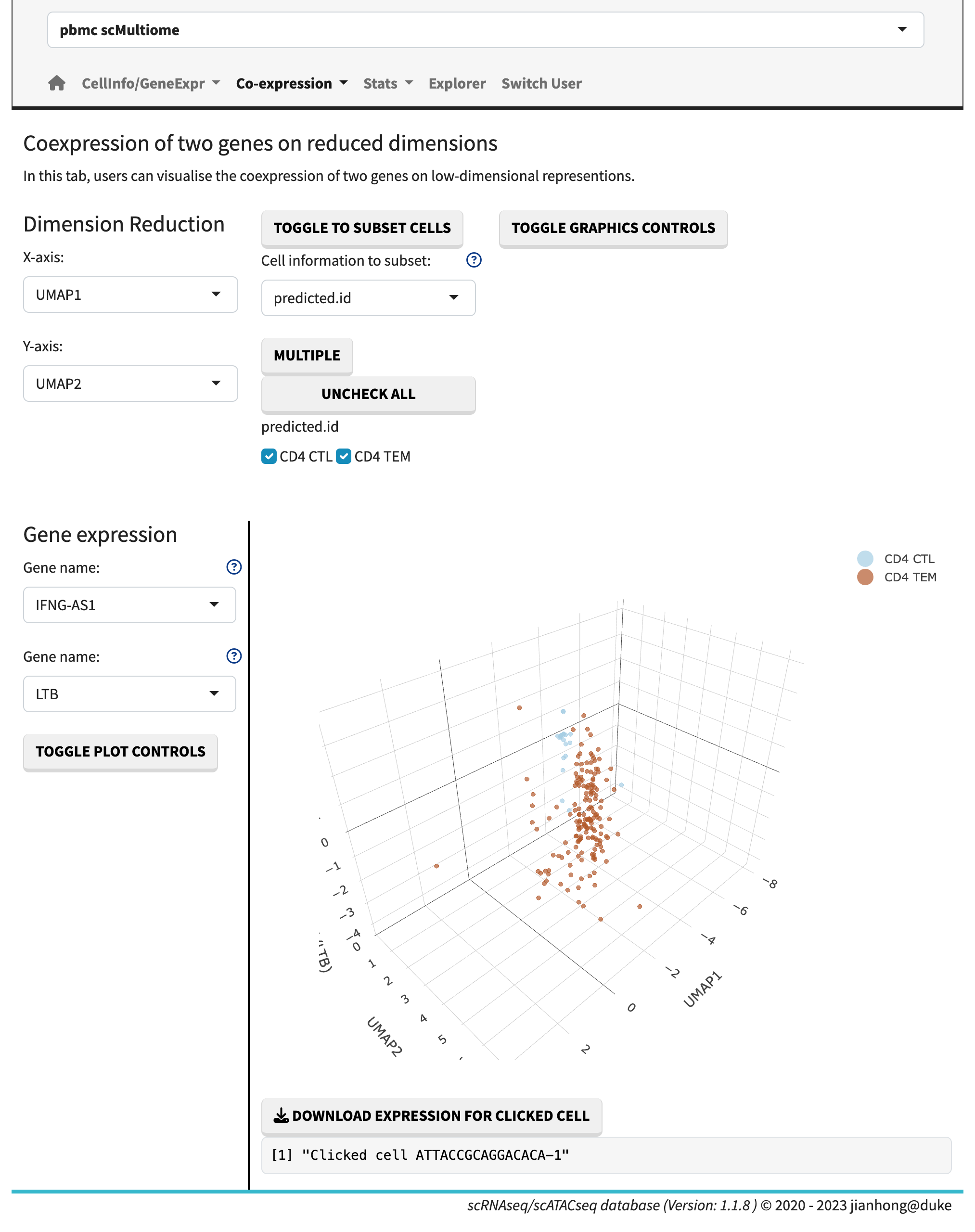
Co-expression 3D plot
- and sunburst plot.
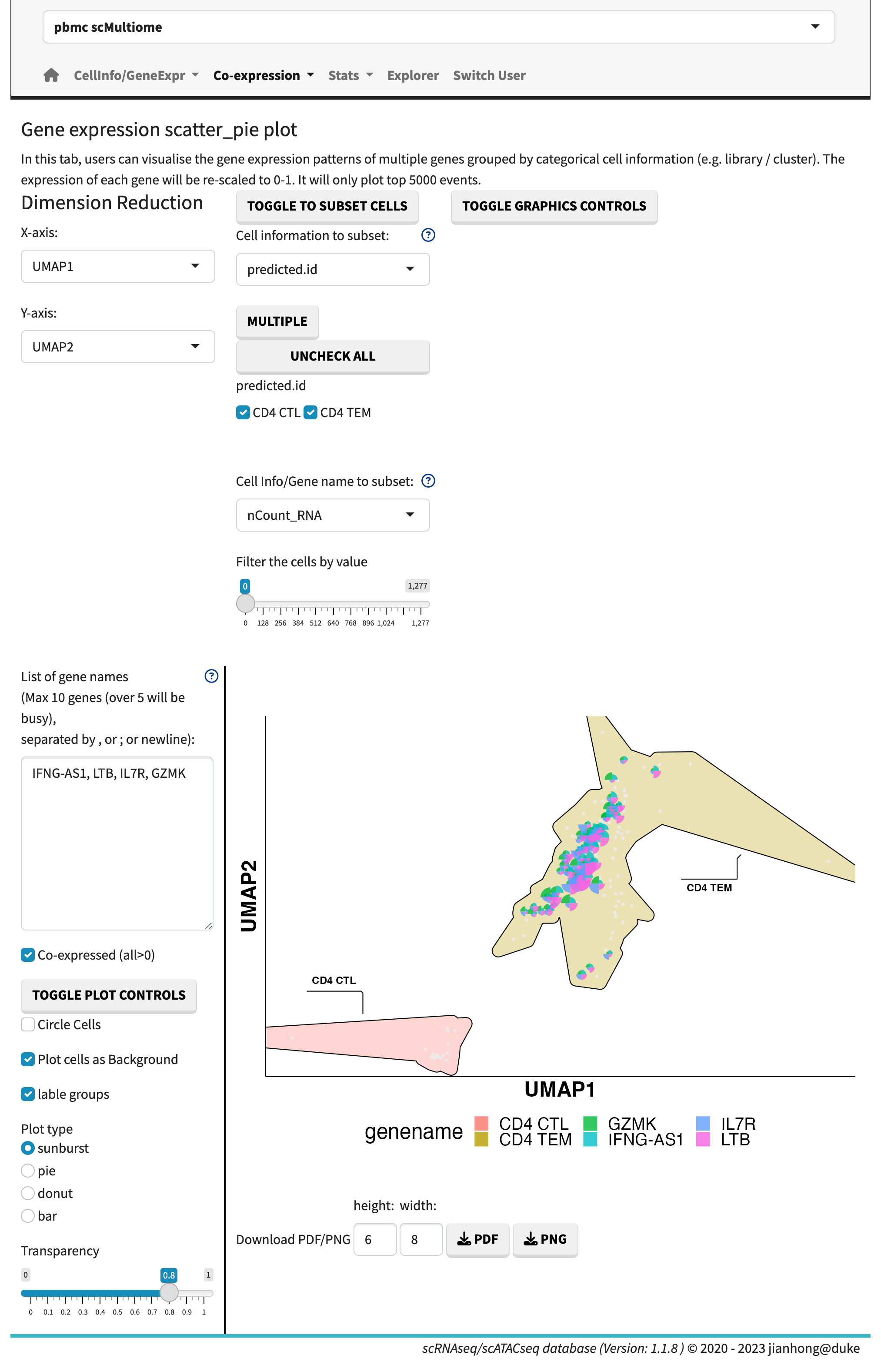
Sunburst plot
In the gene expression vs. gene expression sub-module, the gene expression levels are plotted side by side. The gene co-expression plots showcase the relative expression levels in a 2D or 3D heatmap format. The sunburst plot, on the other hand, enables the visualization of expression levels for more than two genes simultaneously.
Statistical plots
The sub-modules of statistical plots offer a range of visualization options, including violin plots, box plots, proportion plots, bubble plots, heatmaps, and waffle plots.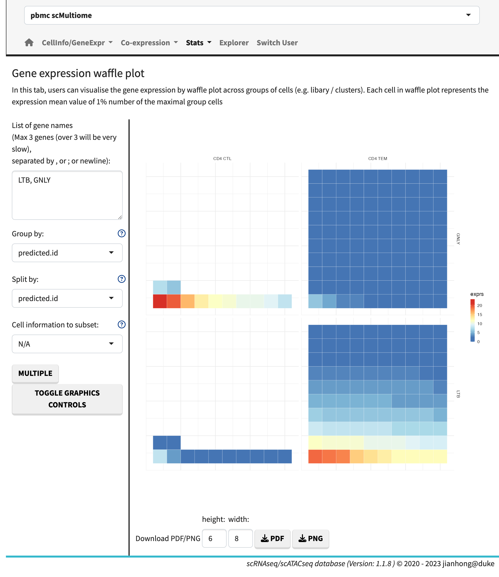
Waffle plot
Within the bubble plot and heatmap sub-module, users have the flexibility to visualize multiple genes across multiple layers, with the option to select violin plots as the plot type. Users can exercise control over various plot parameters, such as changing the order of samples or contents, adjusting the color scheme, and modifying point sizes, among others.
Explorer for multiple combination plots
The Explorer module offers the ability to combine multiple plots within a single page, providing increased flexibility for conducting multiple comparisons. Users can select the module type and click the ‘NEW MODULE’ button to add a plot. The sub-plot modules consist of three regions:
- Icons: These icons allow users to remove a plot, move it down, move it up, and toggle between full width and half width of the window.
- Major Information Dropdown List: This dropdown list provides essential information for the plots.
- Detailed Plot Controllers: These icons offer more specific plot control options.
Users can explore up to eight plots within the module, allowing for a comprehensive analysis within a single interface.
User management
scRNAseqApp borrow the power of shinymanager
package for user management. By default, the scInit
function initial the root user name as “admin” protected with password
“scRNAseqApp”. You can change the root user name and password when you
run scInit or by administrator mode page in
the shiny APP after log in.
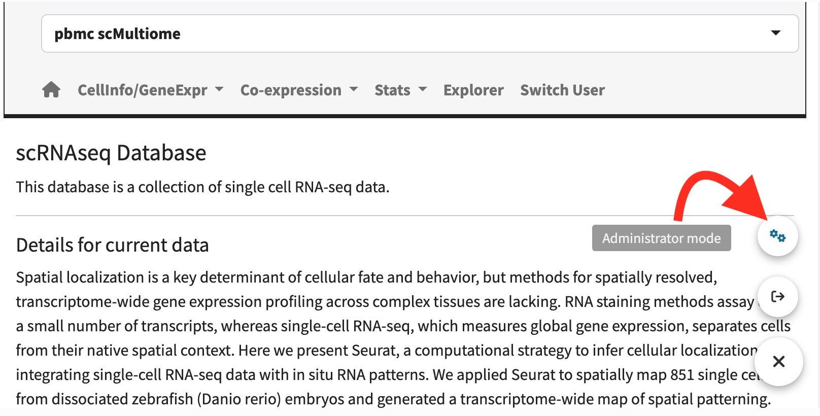
Administrator mode page.
Protect the datasets
To protect unpublished data, simply set the LOCKER
parameter to TRUE when you create the dataset.
pbmc_rds <- system.file("extdata", "pbmc_signac_sub.rds",
                        package="scRNAseqAppBioc2023Workshop",
                        mustWork = TRUE)
pbmc <- readRDS(pbmc_rds)
appconf <- createAppConfig(
  title="pbmc small protected",
  destinationFolder = "pbmc_protected",
  species = "Homo sapiens",
  doi="10.1038/nbt.3192",
  datatype = "scRNAseq")
#> No encoding supplied: defaulting to UTF-8.
createDataSet(appconf, pbmc, LOCKER = TRUE,
              datafolder = file.path(publish_folder, "data"))
#> Loading required package: Signac
#> Centering and scaling data matrix
#> Calculating cluster CD4 TEM
#> For a more efficient implementation of the Wilcoxon Rank Sum Test,
#> (default method for FindMarkers) please install the limma package
#> --------------------------------------------
#> install.packages('BiocManager')
#> BiocManager::install('limma')
#> --------------------------------------------
#> After installation of limma, Seurat will automatically use the more
#> efficient implementation (no further action necessary).
#> This message will be shown once per session
#> Calculating cluster CD4 CTL
#> An object of class Seurat
#> 3786 features across 191 samples within 3 assays
#> Active assay: RNA (267 features, 267 variable features)
#>  2 other assays present: SCT, peaks
#>  2 dimensional reductions calculated: pca, umap
dir(file.path(publish_folder, "data", "pbmc_protected"))
#> [1] "appconf.rds" "LOCKER"      "markers.rds" "sc1conf.rds" "sc1def.rds"
#> [6] "sc1gene.rds" "sc1gexpr.h5" "sc1meta.rds"
scRNAseqApp(app_path = publish_folder)
Administrator can add or remove the protection in the
EditData tab of the administrator mode
page.
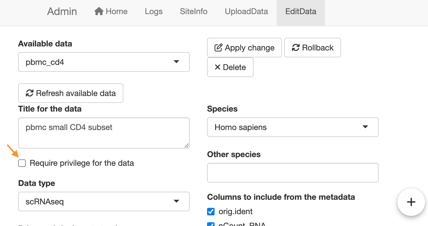
Change the protection status for a data.
Then administrator can add or remove protected data for users in the
Home tab of the administrator mode page.
Please note that the different datasets are separated by ‘;’ in the
Privilege setting.
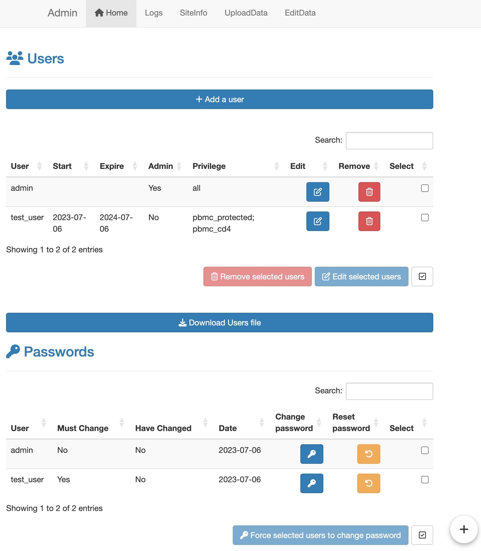
Change the user privileges.
Distribute to a shiny server
There are two steps to distribute to a shiny server. First, install
the package in the server as root user. Second, in a R session run
scInit() after load the scRNAseqApp library.
If you initialed the app offline, copy the app folder to the shiny
server.
Note: the following files need to be writable for shiny:
www/database.sqlite, www/counter.tsv and the
app www folder should also be writable because the user
manager is depend on SQLite, and the SQLite needs to be able to create a
journal file in the same directory as the DB, before any modifications
can take place. The journal is used to support transaction rollback.
Add additional data to the APP
To add additional data to the APP, first prepare an preprocessed
scRNA-Seq data, scATAC-Seq data or scMultiomic data. Then create a
appconf object to include the basic information about the
data. After that use createDataSet to add the data to
publish folder.
Add preprocessed scRNA-Seq data in Seurat format
# just modify the appconf we created in previous step
# the data will write to folder bpmc_cd4 with title 'bpmc small CD4 subset'
appconf$title <- "pbmc small CD4 subset"
appconf$id <- "pbmc_cd4"
createDataSet(appconf, pbmc, datafolder = file.path(publish_folder, "data"))
#> Centering and scaling data matrix
#> Calculating cluster CD4 TEM
#> Calculating cluster CD4 CTL
#> An object of class Seurat
#> 3786 features across 191 samples within 3 assays
#> Active assay: RNA (267 features, 267 variable features)
#>  2 other assays present: SCT, peaks
#>  2 dimensional reductions calculated: pca, umap
dir(file.path(publish_folder, "data", "pbmc_cd4"))
#> [1] "appconf.rds" "markers.rds" "sc1conf.rds" "sc1def.rds"  "sc1gene.rds"
#> [6] "sc1gexpr.h5" "sc1meta.rds"
Add preprocessed scRNA-Seq data in annData format
annData is the data format saved by most of the popular
python based scRNA-seq analysis pipelines. You need to convert the
annData into Seurat object first and then add
the data into the APP. Here are some useful links for that: https://mojaveazure.github.io/seurat-disk/articles/convert-anndata.html
https://github.com/cellgeni/sceasy
Add 10X genomics Chromium Single Cell Multiome ATAC + Gene Expression data
library(SeuratObject)
#> Loading required package: sp
appconf$title <- "pbmc scMultiome"
appconf$id <- "pbmc_multiome"
appconf$type <- "scMultiome"
for(i in seq_along(pbmc@assays$peaks@fragments)){## patch the fragment path
  pbmc@assays$peaks@fragments[[i]]@path <-
    file.path(dirname(pbmc_rds), pbmc@assays$peaks@fragments[[i]]@path)
}
createDataSet(appconf,
              pbmc,
              atacAssayName="peaks",
              datafolder = file.path(publish_folder, "data"))
#> Centering and scaling data matrix
#> Calculating cluster CD4 TEM
#> Calculating cluster CD4 CTL
#> Warning in makeShinyFiles(seu, scConf = config, assayName = assayName, gexSlot
#> = gexSlot, : scATAC links data are not available.
#> The following steps will cost memories.
#> Loading required package: BiocGenerics
#>
#> Attaching package: 'BiocGenerics'
#> The following object is masked from 'package:scRNAseqApp':
#>
#>     lapply
#> The following objects are masked from 'package:stats':
#>
#>     IQR, mad, sd, var, xtabs
#> The following objects are masked from 'package:base':
#>
#>     anyDuplicated, aperm, append, as.data.frame, basename, cbind,
#>     colnames, dirname, do.call, duplicated, eval, evalq, Filter, Find,
#>     get, grep, grepl, intersect, is.unsorted, lapply, Map, mapply,
#>     match, mget, order, paste, pmax, pmax.int, pmin, pmin.int,
#>     Position, rank, rbind, Reduce, rownames, sapply, setdiff, sort,
#>     table, tapply, union, unique, unsplit, which.max, which.min
#> Loading required package: S4Vectors
#> Loading required package: stats4
#>
#> Attaching package: 'S4Vectors'
#> The following object is masked from 'package:utils':
#>
#>     findMatches
#> The following objects are masked from 'package:base':
#>
#>     expand.grid, I, unname
#>
#> Attaching package: 'IRanges'
#> The following object is masked from 'package:sp':
#>
#>     %over%
#> An object of class Seurat
#> 3786 features across 191 samples within 3 assays
#> Active assay: RNA (267 features, 267 variable features)
#>  2 other assays present: SCT, peaks
#>  2 dimensional reductions calculated: pca, umap
dir(file.path(publish_folder, "data", "pbmc_multiome"))
#>  [1] "appconf.rds" "bws"         "markers.rds" "sc1anno.rds" "sc1atac.h5"
#>  [6] "sc1conf.rds" "sc1def.rds"  "sc1gene.rds" "sc1gexpr.h5" "sc1link.rds"
#> [11] "sc1meta.rds" "sc1peak.rds"
Add ArchR or Signac preprocessed scATAC-Seq data
To add ArchR preprocessed data, the first step is to convert it into Signac like Seurat object. Here is the pseudo-code for adding a preprocessed scATAC-Seq data.
library(ArchRtoSignac)
packages <- c("ArchR","Seurat", "Signac","stringr") # required packages
loadinglibrary(packages)
fragments_dirs <- "path/to/fragments/"
proj <- readRDS("path/to/Save-ArchR-Project.rds")
## do this when you moved the Arrow files
## skip it if you did not change the directory of your Arrow files.
proj@sampleColData$ArrowFiles <- sub("previouse/dirname/to/ArrowFiles",
                                     "current/dirname/to/ArrowFiles",
                                     proj@sampleColData$ArrowFiles)
proj@projectMetadata$outputDirectory <- "path/to/metadata/output/dir"
pkm <- getPeakMatrix(proj) # proj is an ArchRProject
getAvailableMatrices(proj)
library(EnsDb.Mmusculus.v79) # if it is a mouse data (mm10)
annotations <- getAnnotation(reference = EnsDb.Mmusculus.v79, refversion = "mm10")
ArchR2Signac <- function (ArchRProject, refversion, samples = NULL, fragments_dir = NULL,
          pm, fragments_fromcellranger = NULL, fragments_file_extension = NULL,
          annotation, validate.fragments = FALSE){
  if (is.null(samples)) {
    samples <- unique(ArchRProject@cellColData$Sample)
  }
  if (fragments_fromcellranger == "YES" | fragments_fromcellranger ==
      "Y" | fragments_fromcellranger == "Yes") {
    print("In Progress:")
    print("Prepare Seurat list for each sample")
    output_dir = "/outs/"
    seurat_list <- lapply(samples, function(cur_sample) {
      print(cur_sample)
      cur_fragments <- ifelse(is.list(fragments_dir), paste0(fragments_dir[[which(samples ==
                                                                                    cur_sample)]], output_dir, "fragments.tsv.gz"),
                              paste0(fragments_dir, cur_sample, output_dir,
                                     "fragments.tsv.gz"))
      cur_pm <- pm[, grepl(paste0(cur_sample, "#"), colnames(pm))]
      cur_meta <- ArchRProject@cellColData %>% as.data.frame %>%
        subset(Sample == cur_sample)
      colnames(cur_pm) <- do.call(rbind, str_split(colnames(cur_pm),
                                                   "#"))[, 2]
      rownames(cur_meta) <- do.call(rbind, str_split(rownames(cur_meta),
                                                     "#"))[, 2]
      print(dim(cur_pm))
      cur_chromatin <- Signac::CreateChromatinAssay(counts = cur_pm,
                                                    sep = c("-", "-"), fragments = cur_fragments,
                                                    ranges = ArchRProject@peakSet, genome = refversion,
                                                    annotation = annotation)
      cur_atac <- Seurat::CreateSeuratObject(cur_chromatin,
                                             assay = "peaks", meta.data = cur_meta, )
    })
  }
  if (fragments_fromcellranger == "NO" | fragments_fromcellranger ==
      "N" | fragments_fromcellranger == "No") {
    print("IF selecting NO, please make sure to provide fragments_file_extension")
    print("In Progress:")
    print("Prepare Seurat list for each sample")
    seurat_list <- lapply(samples, function(cur_sample) {
      print(cur_sample)
      cur_fragments <- ifelse(is.list(fragments_dir), paste0(fragments_dir[[which(samples ==
                                                                                    cur_sample)]], fragments_file_extension), paste0(fragments_dir,
                                                                                                                                     cur_sample, fragments_file_extension))
      cur_pm <- pm[, grepl(paste0(cur_sample, "#"), colnames(pm))]
      cur_meta <- ArchRProject@cellColData %>% as.data.frame %>%
        subset(Sample == cur_sample)
      colnames(cur_pm) <- do.call(rbind, str_split(colnames(cur_pm),
                                                   "#"))[, 2]
      rownames(cur_meta) <- do.call(rbind, str_split(rownames(cur_meta),
                                                     "#"))[, 2]
      print(dim(cur_pm))
      cur_chromatin <- Signac::CreateChromatinAssay(counts = cur_pm,
                                                    sep = c("-", "-"), fragments = cur_fragments,
                                                    ranges = ArchRProject@peakSet, genome = refversion,
                                                    annotation = annotation,
                                                    validate.fragments = validate.fragments)
      cur_atac <- Seurat::CreateSeuratObject(cur_chromatin,
                                             assay = "peaks", meta.data = cur_meta, )
    })
  }
  print("In Progress:")
  print("Merge Seurat list")
  SeuratObject <- merge(x = seurat_list[[1]], y = seurat_list[2:length(seurat_list)],
                        add.cell.ids = samples)
  print("Return SeuratObject")
  SeuratObject
}

seurat_atac <- ArchR2Signac(
  ArchRProject = proj,
  refversion = "mm10",
  #samples = samplelist, # list of samples in the ArchRProject (default will use ArchRProject@cellColData$Sample but another list can be provided)
  fragments_dir = fragments_dirs,
  pm = pkm, # peak matrix from getPeakMatrix()
  fragments_fromcellranger = "No", # fragments_fromcellranger This is an Yes or No selection ("NO" | "N" | "No" or "YES" | "Y" | "Yes")
  fragments_file_extension = ".tsv.gz", # Default - NULL: File_Extension for fragments files (typically they should be '.tsv.gz' or '.fragments.tsv.gz')
  annotation = annotations # annotation from getAnnotation()
)

gsm <- getGeneScoreMatrix(ArchRProject = proj, SeuratObject = seurat_atac)

seurat_atac[['RNA']] <- CreateAssayObject(counts = gsm)

seurat_atac <- addDimRed(
  ArchRProject = proj,
  SeuratObject = seurat_atac,
  addUMAPs = "UMAP",
  reducedDims = "IterativeLSI"
) # default is "IterativeLSI"

#add both 'Harmony' and ‘IterativeLSI’:
seurat_atac <- addTwoDimRed(
  ArchRProject = proj,
  SeuratObject = seurat_atac,
  addUMAPs = "UMAP",
  reducedDims1 = "IterativeLSI",
  # Please limit your reducedDims to one of the following: IterativeLSI, IterativeLSI2 or Harmony
  reducedDims2 = "Harmony" # IterativeLSI2 or Harmony
)
appconf <- createAppConfig(
       title="scATACseq example",
       destinationFolder = "scATACseq_exp",
       species = "Mus musculus",
       datatype = "scATAC")
createDataSet(appconf, seurat_atac, atacAssayName="peaks", file.path(publish_folder, "data"))

scRNAseqApp()
SessionInfo
sessionInfo()
#> R version 4.3.1 (2023-06-16)
#> Platform: x86_64-pc-linux-gnu (64-bit)
#> Running under: Ubuntu 22.04.2 LTS
#>
#> Matrix products: default
#> BLAS:   /usr/lib/x86_64-linux-gnu/openblas-pthread/libblas.so.3
#> LAPACK: /usr/lib/x86_64-linux-gnu/openblas-pthread/libopenblasp-r0.3.20.so;  LAPACK version 3.10.0
#>
#> locale:
#>  [1] LC_CTYPE=en_US.UTF-8       LC_NUMERIC=C
#>  [3] LC_TIME=en_US.UTF-8        LC_COLLATE=en_US.UTF-8
#>  [5] LC_MONETARY=en_US.UTF-8    LC_MESSAGES=en_US.UTF-8
#>  [7] LC_PAPER=en_US.UTF-8       LC_NAME=C
#>  [9] LC_ADDRESS=C               LC_TELEPHONE=C
#> [11] LC_MEASUREMENT=en_US.UTF-8 LC_IDENTIFICATION=C
#>
#> time zone: Etc/UTC
#> tzcode source: system (glibc)
#>
#> attached base packages:
#> [1] stats4    stats     graphics  grDevices utils     datasets  methods
#> [8] base
#>
#> other attached packages:
#> [1] GenomeInfoDb_1.37.2 IRanges_2.35.2      S4Vectors_0.39.1
#> [4] BiocGenerics_0.47.0 SeuratObject_4.1.3  sp_2.0-0
#> [7] Signac_1.10.0       scRNAseqApp_1.1.9   pander_0.6.5
#>
#> loaded via a namespace (and not attached):
#>   [1] TrajectoryUtils_1.9.0       RcppAnnoy_0.0.21
#>   [3] slingshot_2.9.0             splines_4.3.1
#>   [5] later_1.3.1                 BiocIO_1.11.0
#>   [7] bitops_1.0-7                R.oo_1.25.0
#>   [9] tibble_3.2.1                polyclip_1.10-4
#>  [11] XML_3.99-0.14               shinymanager_1.0.410
#>  [13] lifecycle_1.0.3             doParallel_1.0.17
#>  [15] rprojroot_2.0.3             hdf5r_1.3.8
#>  [17] globals_0.16.2              lattice_0.21-8
#>  [19] MASS_7.3-60                 backports_1.4.1
#>  [21] magrittr_2.0.3              plotly_4.10.2
#>  [23] sass_0.4.7                  rmarkdown_2.23
#>  [25] jquerylib_0.1.4             yaml_2.3.7
#>  [27] httpuv_1.6.11               Seurat_4.3.0.1
#>  [29] sctransform_0.3.5           askpass_1.1
#>  [31] spatstat.sparse_3.0-2       reticulate_1.30
#>  [33] DBI_1.1.3                   cowplot_1.1.1
#>  [35] pbapply_1.7-2               RColorBrewer_1.1-3
#>  [37] lubridate_1.9.2             abind_1.4-5
#>  [39] zlibbioc_1.47.0             Rtsne_0.16
#>  [41] GenomicRanges_1.53.1        R.utils_2.12.2
#>  [43] purrr_1.0.1                 RCurl_1.98-1.12
#>  [45] tweenr_2.0.2                circlize_0.4.15
#>  [47] GenomeInfoDbData_1.2.10     ggrepel_0.9.3
#>  [49] irlba_2.3.5.1               listenv_0.9.0
#>  [51] spatstat.utils_3.0-3        goftest_1.2-3
#>  [53] spatstat.random_3.1-5       fitdistrplus_1.1-11
#>  [55] parallelly_1.36.0           pkgdown_2.0.7
#>  [57] RcppRoll_0.3.0              leiden_0.4.3
#>  [59] codetools_0.2-19            DelayedArray_0.27.10
#>  [61] DT_0.28                     xml2_1.3.5
#>  [63] ggforce_0.4.1               tidyselect_1.2.0
#>  [65] shape_1.4.6                 farver_2.1.1
#>  [67] matrixStats_1.0.0           spatstat.explore_3.2-1
#>  [69] GenomicAlignments_1.37.0    jsonlite_1.8.7
#>  [71] GetoptLong_1.0.5            ellipsis_0.3.2
#>  [73] progressr_0.13.0            ggridges_0.5.4
#>  [75] survival_3.5-5              iterators_1.0.14
#>  [77] systemfonts_1.0.4           foreach_1.5.2
#>  [79] tools_4.3.1                 ragg_1.2.5
#>  [81] ica_1.0-3                   Rcpp_1.0.11
#>  [83] glue_1.6.2                  gridExtra_2.3
#>  [85] SparseArray_1.1.11          RefManageR_1.4.0
#>  [87] xfun_0.39                   MatrixGenerics_1.13.1
#>  [89] dplyr_1.1.2                 withr_2.5.0
#>  [91] fastmap_1.1.1               fansi_1.0.4
#>  [93] openssl_2.1.0               digest_0.6.33
#>  [95] timechange_0.2.0            R6_2.5.1
#>  [97] mime_0.12                   textshaping_0.3.6
#>  [99] colorspace_2.1-0            scattermore_1.2
#> [101] tensor_1.5                  RSQLite_2.3.1
#> [103] spatstat.data_3.0-1         R.methodsS3_1.8.2
#> [105] utf8_1.2.3                  tidyr_1.3.0
#> [107] generics_0.1.3              data.table_1.14.8
#> [109] rtracklayer_1.61.0          httr_1.4.6
#> [111] htmlwidgets_1.6.2           S4Arrays_1.1.5
#> [113] uwot_0.1.16                 pkgconfig_2.0.3
#> [115] gtable_0.3.3                blob_1.2.4
#> [117] ComplexHeatmap_2.17.0       lmtest_0.9-40
#> [119] SingleCellExperiment_1.23.0 XVector_0.41.1
#> [121] htmltools_0.5.5             shinyhelper_0.3.2
#> [123] bookdown_0.34               clue_0.3-64
#> [125] scales_1.2.1                Biobase_2.61.0
#> [127] png_0.1-8                   ggdendro_0.1.23
#> [129] knitr_1.43                  reshape2_1.4.4
#> [131] rjson_0.2.21                curl_5.0.1
#> [133] nlme_3.1-162                cachem_1.0.8
#> [135] zoo_1.8-12                  GlobalOptions_0.1.2
#> [137] stringr_1.5.0               KernSmooth_2.23-22
#> [139] parallel_4.3.1              miniUI_0.1.1.1
#> [141] restfulr_0.0.15             desc_1.4.2
#> [143] pillar_1.9.0                grid_4.3.1
#> [145] vctrs_0.6.3                 RANN_2.6.1
#> [147] promises_1.2.0.1            princurve_2.1.6
#> [149] billboarder_0.4.0           xtable_1.8-4
#> [151] cluster_2.1.4               evaluate_0.21
#> [153] cli_3.6.1                   compiler_4.3.1
#> [155] Rsamtools_2.17.0            rlang_1.1.1
#> [157] crayon_1.5.2                sortable_0.5.0
#> [159] future.apply_1.11.0         plyr_1.8.8
#> [161] fs_1.6.3                    stringi_1.7.12
#> [163] viridisLite_0.4.2           deldir_1.0-9
#> [165] BiocParallel_1.35.3         assertthat_0.2.1
#> [167] munsell_0.5.0               Biostrings_2.69.2
#> [169] lazyeval_0.2.2              spatstat.geom_3.2-4
#> [171] Matrix_1.6-0                scrypt_0.1.6
#> [173] patchwork_1.1.2             bit64_4.0.5
#> [175] future_1.33.0               learnr_0.11.4
#> [177] ggplot2_3.4.2               shiny_1.7.4.1
#> [179] highr_0.10                  SummarizedExperiment_1.31.1
#> [181] ROCR_1.0-11                 igraph_1.5.0.1
#> [183] memoise_2.0.1               bslib_0.5.0
#> [185] bibtex_0.5.1                fastmatch_1.1-3
#> [187] bit_4.0.5