Introduction
The lollipop-style or needle-style plot are often used for displaying the distribution of mutations or genetic variations along with a variety of genomic annotations, such as gene models and CpG island. Several tools provide lollipop-style plot to show the mutation data such as cBioPortal Tools::MutationMapper1, EMBL-EBI::Pfam2, BioJS::muts-needle-plot3, BiQ Analyzer4, and Methylation plotter5. The cBioPortal Tools::MutationMapper is a well-known and easy to use on-line genome browser that can output high quality of figures with mutations with tab-delimited mutation data. In R/Bioconductor, there are options to use the flexibility of the Rgraphics system to display Methylation data such as MethVisual6 and GenVisR7.
Table 1: Tools availble for lollipop plot.
| software | inputs | online | description |
|---|---|---|---|
| MutationMapper1 | tab-delimited text | Yes | interprets mutations with different heights along protein annotations in automatic color theme |
| Pfam2 | JSON | Yes | could combine different line and head colors with different drawing styles |
| muts-needle-plot3 | JSON | No | plots data point with different colors, heights, and size along annotations, and highlighted selcted coordinates |
| BiQ Analyzer4 | BiQ methylation file | Yes | interprets methylation status in black & white |
| Methylation plotter5 | tab-delimited text | Yes | stacked multiple methylation status for multiple samples |
| MethVisual6 | R list | No | visualize the methylation status of CpGs according to their genomic position |
| REDseq8 | R list | No | plot frequencies of methylations and SNPs along a chromosome |
| GenVisR7 | R dataframe | No | plot most accurate graphic representation of the ensembl annotation version based on biomart service |
However, when mutations/SNPs are densely distributed, figures generated by the above tools can become cluttered and unreadable.To fill this gap, we developed trackViewer, an R/Bioconductor package as an enhanced light-weight genome viewer for visualizing various types of high-throughput sequencing data, side by side or stacked with multiple annotation tracks. Besides the regular read coverage tracks supported by existing genome browsers/viewers, trackViewer can also be used to generate lollipop and dandeline plot to depict the sparse or dense methylation and SNP/mutation status, together with coverage data and annotation tracks to facilitate integrated analysis of multi-omics data. In addition, figures generated by trackViewer are interactive, i.e., the feel-and-look such as the layout, the color scheme, and the order of tracks can be easily customized by the users. Furthermore, trackViewer can be easily integrated into standard analysis pipeline for various high-throughput sequencing dataset such as ChIP-seq, RNA-seq, methylation-seq or DNA-seq. The images produced by trackViewer are highly customizable including labels, symbols, colors, and size. Here, we illustrate its utilities and capabilities in deriving biological insights from multi-omics dataset from GEO/Encode.
Installation
BiocManager is used to install the released version of trackViewer.
To check the current version of trackViewer, please try
packageVersion("trackViewer")## [1] '1.27.14'Quick guide for generating lollipop plots using the lolliplot function in trackViewer package.
Step 1. Prepare the methylation/variant/mutation data
The input data for the lolliplot function in trackViewer is an object of GenomicRanges::GRanges.
## load library
library(trackViewer)
set.seed(123) ## set the seed to make sure the analysis can be repeated.
## SNP locations to be randomly sampled
SNP <- c(10, 100, 105, 108, 400, 410, 420, 600, 700, 805, 840, 1400, 1402)
## use GenomicRanges::GRanges function to create a GRanges object.
## For real data, users can import vcf data via VariantAnnotation::readVcf function.
sample.gr <- GRanges("chr1", IRanges(SNP, width=1,
                     ## the name of GRanges object will be used as label
                     names=paste0("snp", SNP)),
                     ## the score value will be used as the height of lollipop
                     score = sample.int(5, length(SNP), replace = TRUE),
                     ## set the color for lollipop node.
                     color = sample.int(6, length(SNP), replace = TRUE),
                     ## set the color fot the lollipop stem
                     border = sample(c("black", "gray80", "gray30"),
                                     length(SNP), replace=TRUE)
                     )
Step 2. Prepare the gene/protein model
The gene/protein model for the lolliplot function by trackViewer is also an object of GenomicRanges::GRanges.
Step 3. Plot lollipop plot using the lolliplot function
Densely distributed SNPs/mutations is displayed side-by-side with jittered positions.
lolliplot(sample.gr, features.gr)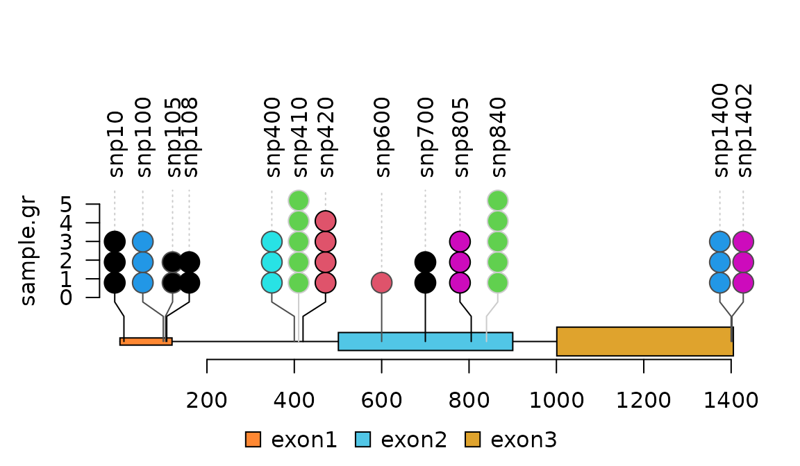
Plot data in Variant Call Format (VCF)
VCF is a text file format is a text format for storing gene sequence variations such as genomic positions, original genotypes, and optional genotypes. The trackViewer package can be used to display single nucleotide polymorphisms (SNPs) in VCF file as lollipop-style plots. The input data for the folloiwng example are variant data from chromosome 22 in the 1000 Genomes project which is included in the VariantAnnotation package.
Note that the number of circles indicates the number of SNP events. Different colors differentiate known SNPs from new mutation events.
library(VariantAnnotation) ## load the package for reading the vcf file
library(TxDb.Hsapiens.UCSC.hg19.knownGene) ## load the package for obtaining the gene model
library(org.Hs.eg.db) ## load the package for fetching the gene name
library(rtracklayer)
fl <- system.file("extdata", "chr22.vcf.gz", package="VariantAnnotation")
## set the track range
gr <- GRanges("22", IRanges(50968014, 50970514, names="TYMP"))
## read in the vcf file
tab <- TabixFile(fl)
vcf <- readVcf(fl, "hg19", param=gr)
## get GRanges from the VCF object
mutation.frequency <- rowRanges(vcf)
## keep the metadata
mcols(mutation.frequency) <-
    cbind(mcols(mutation.frequency),
          VariantAnnotation::info(vcf))
## set colors
mutation.frequency$border <- "gray30"
mutation.frequency$color <-
    ifelse(grepl("^rs", names(mutation.frequency)),
           "lightcyan", "lavender")
## plot Global Allele Frequency based on AC/AN
mutation.frequency$score <- round(mutation.frequency$AF*100)
## change the rotation angle of the SNP label
mutation.frequency$label.parameter.rot <- 45
## keep the sequence level style to UCSC
seqlevelsStyle(gr) <- seqlevelsStyle(mutation.frequency) <- "UCSC"
seqlevels(mutation.frequency) <- "chr22"
## extract transcripts in the given ranges
trs <- geneModelFromTxdb(TxDb.Hsapiens.UCSC.hg19.knownGene,
                         org.Hs.eg.db, gr=gr)
## subset the features to show the transcripts of your interest only
features <- c(range(trs[[1]]$dat), range(trs[[5]]$dat))
## define the feature labels
names(features) <- c(trs[[1]]$name, trs[[5]]$name)
## define the feature colors
features$fill <- c("lightblue", "mistyrose")
## define the feature heights
features$height <- c(.02, .04)
## set the legends
legends <- list(labels=c("known", "unkown"),
                fill=c("lightcyan", "lavender"),
                color=c("gray80", "gray80"))
## lollipop plot
lolliplot(mutation.frequency,
          features, ranges=gr, type="circle",
          legend=legends)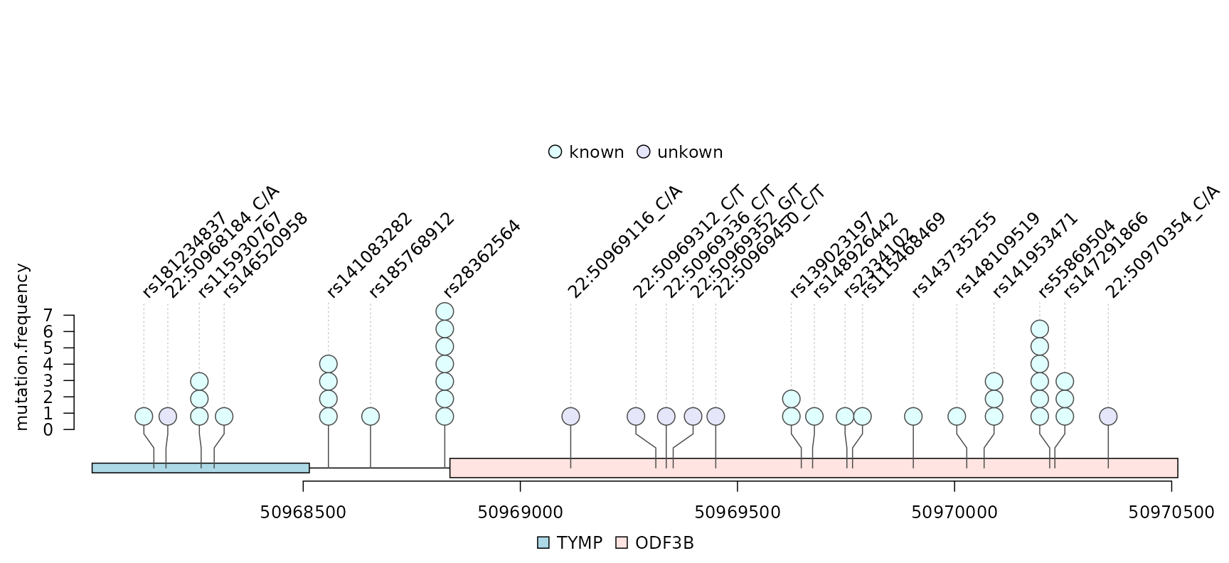
lollipop plot for VCF data
Plot methylation data from files in bed format
Any data that can be imported into a GRanges object can be viewed by trackViewer package. In the following example, we will illustrate how to plot methylation data in bed format.
First, the rtracklayer package is used to import the methylation data into a GRanges. Then, the transcripts are extracted from the TxDb object with gene symbol annotated using the org database. In addition, multiple transcripts can be shown in different colors and tracks.
library(TxDb.Hsapiens.UCSC.hg19.knownGene) ## load the package for obtaining the gene model
library(org.Hs.eg.db) ## load the package for fetching the gene name
library(rtracklayer)
## set the track range
gr <- GRanges("chr22", IRanges(50968014, 50970514, names="TYMP"))
## extract transcripts in given ranges
trs <- geneModelFromTxdb(TxDb.Hsapiens.UCSC.hg19.knownGene,
                         org.Hs.eg.db, gr=gr)
## subset the features to show the transcripts of your interest
features <- GRangesList(trs[[1]]$dat, trs[[5]]$dat, trs[[6]]$dat)
flen <- elementNROWS(features)
features <- unlist(features)
## define feature track layers
features$featureLayerID <- rep(1:2, c(sum(flen[-3]), flen[3]))
## define feature labels
names(features) <- features$symbol
## define feature colors
features$fill <- rep(c("lightblue", "mistyrose", "mistyrose"), flen)
## define feature heights
features$height <- ifelse(features$feature=="CDS", .04, .02)
## import methylation data from a file in bed format
methy <- import(system.file("extdata", "methy.bed", package="trackViewer"), "BED")
## filter the data
methy <- methy[methy$score > 20]
## Please note that for pie plot, there must be at least two numeric columns
methy$score2 <- max(methy$score) - methy$score
## set the legends
legends <- list(labels=c("methylated", "unmethylated"),
                fill=c("white", "lightblue"),
                color=c("black", "black"))
## lollipop plot in pie layout
lolliplot(methy, features,
          ranges=gr, type="pie",
          legend=legends)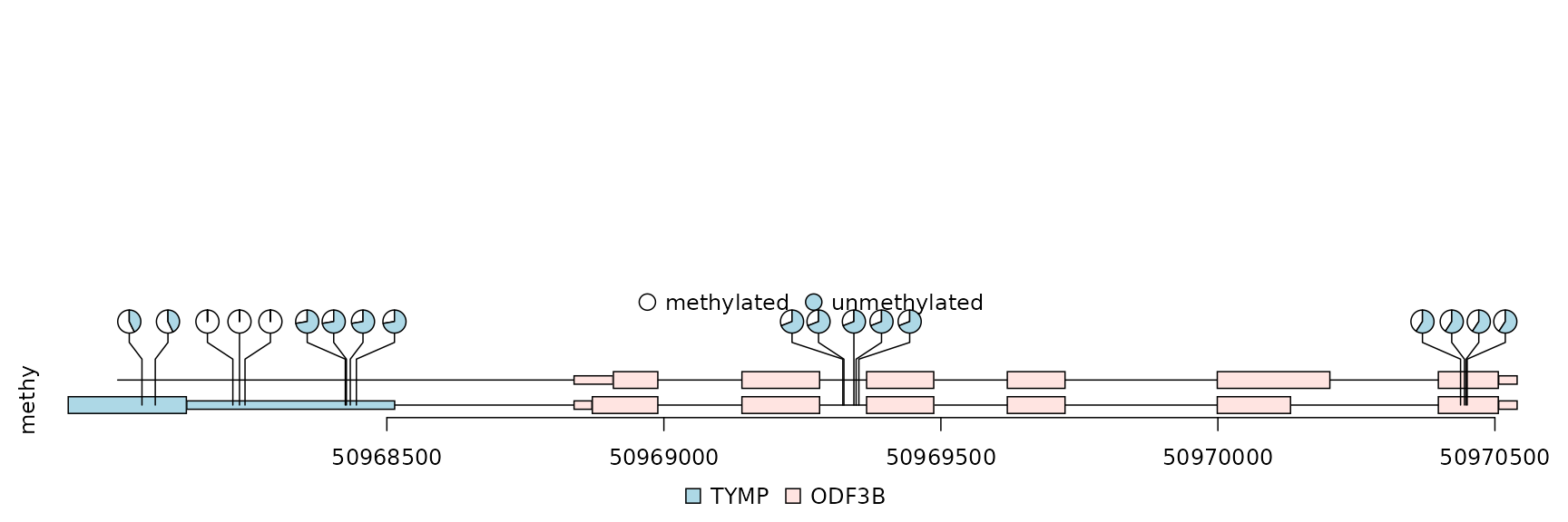
lollipop plot, pie layout
Plot lollipop plot for multiple patients in “pie.stack” layout
The percentage of methylation rates can be shown in pie chart with different layers for different patients.
## simulate multiple patients
rand.id <- sample.int(length(methy), 3*length(methy), replace=TRUE)
rand.id <- sort(rand.id)
methy.mul.patient <- methy[rand.id]
## Please note that pie.stack requires metadata "stack.factor", score, and score2. In addtion,
## the metadata cannot contain stack.factor.order or stack.factor.first for pie.stack style.
len.max <- max(table(rand.id))
stack.factors <- paste0("patient",
                        formatC(1:len.max,
                                width=nchar(as.character(len.max)),
                                flag="0"))
methy.mul.patient$stack.factor <-
    unlist(lapply(table(rand.id), sample, x=stack.factors))
methy.mul.patient$score <-
    sample.int(100, length(methy.mul.patient), replace=TRUE)
## for a pie plot, two or more numeric meta-columns are required.
methy.mul.patient$score2 <- 100 - methy.mul.patient$score
## set different color set for different patient
patient.color.set <- as.list(as.data.frame(rbind(rainbow(length(stack.factors)),
                                                 "#FFFFFFFF"),
                                           stringsAsFactors=FALSE))
names(patient.color.set) <- stack.factors
methy.mul.patient$color <-
    patient.color.set[methy.mul.patient$stack.factor]
## set the legends
legends <- list(labels=stack.factors, col="gray80",
                fill=sapply(patient.color.set, `[`, 1))
## lollipop plot
lolliplot(methy.mul.patient,
          features, ranges=gr,
          type="pie.stack",
          legend=legends)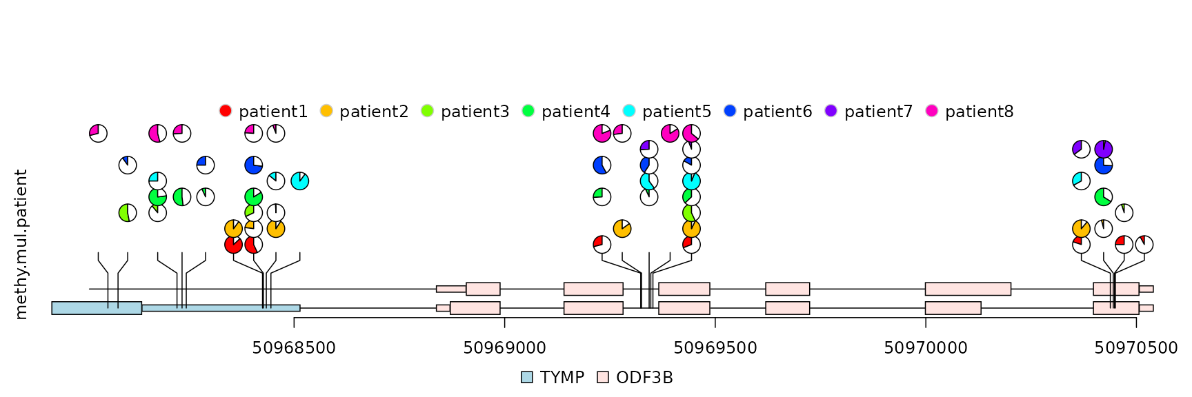
lollipop plot, pie.stack layout
Plot lollipop plot in caterpillar layout to faciliate the comparison between two samples
The caterpillar layout can be used to visualize multiple samples side by side or to display dense data.
## use SNPsideID to separate samples or densely distributed SNPs/mutations/methylation events
sample.gr$SNPsideID <- sample(c("top", "bottom"),
                               length(sample.gr),
                               replace=TRUE)
lolliplot(sample.gr, features.gr)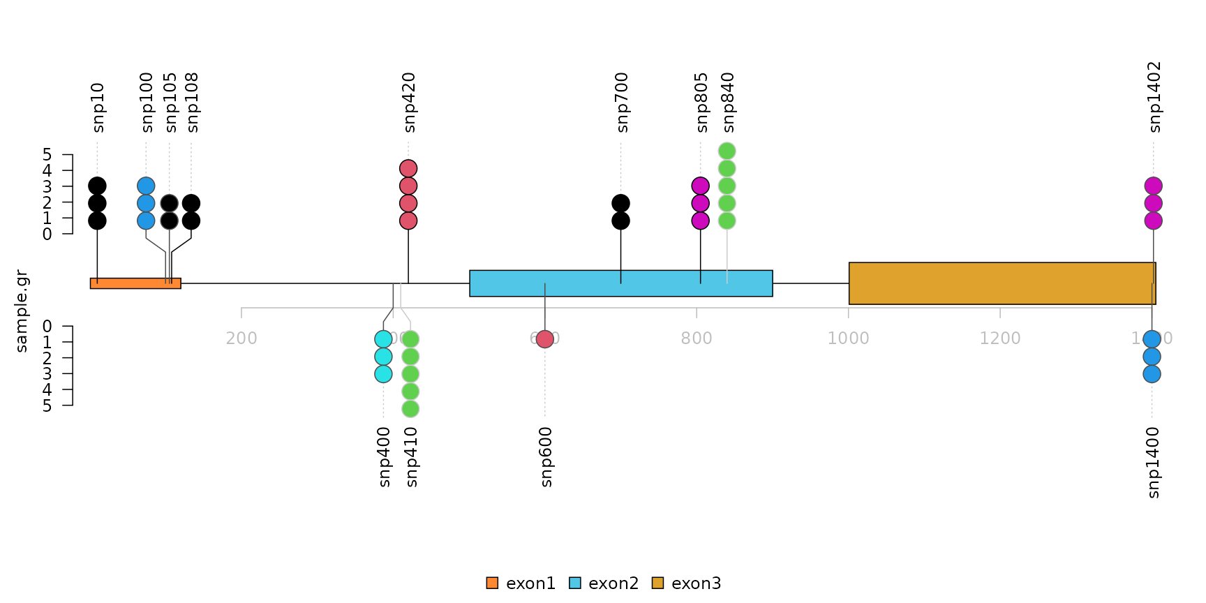
lollipop plot, caterpillar layout
Dandelion plot for the visualization of data with densely distributed SNPs/mutations/methylation events.
Sometimes, there are as many as hundreds of SNPs or methylation status in one gene. Dandelion plot can be used to depict such dense SNPs or methylation events. Please note that the height of the dandelion indicates the density of the events.
methy <- import(system.file("extdata", "methy.bed", package="trackViewer"), "BED")
length(methy)
## [1] 38
## set the color of dandelion leaves.
methy$color <- 3
methy$border <- "gray"
## The following normalization assumes that the total number of events (methy + unmethy) are the same across differnt genomic locations and the ones with the highest score has 100% methylation rate. This is for illustation purpose. For your own data, you will need to calculate the score using methylated/(methylated + unmethylated) for each position.
## rescale the methylation score using the max value of the score
m <- max(methy$score)
methy$score <- methy$score/m
# The area of the fan indicates the percentage of methylation or rate of mutation.
dandelion.plot(methy, features, ranges=gr, type="fan")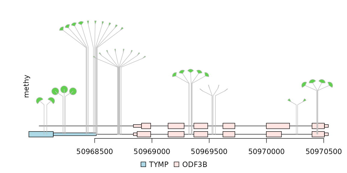
dandelion plot