Scripts for RNA-seq and ChIP-seq analysis primer

Learning Objectives:

pipeline: kallisto and Salmon + tximport + DESeq2 for RNA-seq
pipeline: bwa + MACS2 for ChIP-seq

For more information please refer to the slides

Set-up

All the materials used in this workshop is included in Docker file: jianhong/genomictools

Before we start, please download Docker and install Docker Desktop.

Install docker

Once the docker installed on you system, please try to run the following code in a terminal. This script will get the latest version of docker container for this workshop.

which docker
#docker pull jianhong/genomictools:latest
docker pull ghcr.io/jianhong/genomictools:latest

Change the docker Memory Resources to >= 5G in the Preferences setting page of Docker. And then run the following code in a terminal.

## set docker memory to > 5G
## set docker memory to > 5G ; !important
## RStudio server will not work for M1 chip MacBook.
cd ~
mkdir tmp4genomictools
docker run --memory 5g -e PASSWORD=123456 -p 8787:8787 \
  -v ${PWD}/tmp4genomictools:/home/rstudio/data \
  jianhong/genomictools:latest

“docker run” will open port 8787 on your system. Now you can login rstudio in the container at http://localhost:8787 with username “rstudio” and password “123456”. All the following steps are running in Rstudio “Terminal” or “Console”.

You may want to open the source of “scripts.Rmd” at the “Source Panes” by

rstudioapi::documentOpen("/usr/local/lib/R/site-library/basicBioinformaticsDRC2024/doc/scripts.Rmd")

Run kallisto and Salmon for RNA-seq

The sample files are packaged in basicBioinformaticsDRC2024 package and Docker container.

Now we will download the zebrafish cDNA files from ENSEMBL in order to build the Kallisto and Salmon transcript index. If you are doing rRNA depletion library, please download and merge the cDNA and ncDNA files from ENSEMBL to make the full transcriptome.

cd RNAseq
wget ftp://ftp.ensembl.org/pub/release-105/fasta/danio_rerio/cdna/Danio_rerio.GRCz11.cdna.all.fa.gz

Now we can build the transcriptome index. It will take some time and memory for full dataset. This is the reason why we need to set docker memory to > 5G.

kallisto index -i danRer.GRCz11_transcrits.idx Danio_rerio.GRCz11.cdna.all.fa.gz

salmon index -i danRer.GRCz11_transcrits.salmon.idx -t Danio_rerio.GRCz11.cdna.all.fa.gz

The data are only a subset of the whole genome. We will only use genes in chromosome 4, 13, 16 and 21 to speed up the test run.

mkdir data/RNAseq
cd data/RNAseq
# wget https://raw.githubusercontent.com/jianhong/genomictools/master/inst/extdata/Danio_rerio.GRCz11.cdna.toy.fa.gz
ln -s /usr/local/lib/R/site-library/basicBioinformaticsDRC2024/extdata/Danio_rerio.GRCz11.cdna.toy.fa.gz ./

It will take several seconds to build the toy index.

kallisto index -i danRer.GRCz11_transcrits.toy.idx Danio_rerio.GRCz11.cdna.toy.fa.gz

salmon index -i danRer.GRCz11_transcrits.toy.salmon.idx -t Danio_rerio.GRCz11.cdna.toy.fa.gz

It’s time for quantifying the FASTQ files against our Kallisto index and Salmon index. We run both of them for comparison. For real data, you can select one of them.

Because our FASTQ files are single end reads, we need to set –single for kallisto. And we also need to give the fragment length and standard error of the length for kallisto.

For Salmon, now we can set library type to “A”.

In this example, we put “-t 2” and “-p 2” so we can use up to two processors in the bootstrapping. We set the bootstrapping by “-b 30” and “–numBootstraps 30”.

It will take several minutes for the sample data.

# the toy RNAseq data is saved in /home/rstudio/RNAseq folder
# create a link to current folder
ln -s /home/rstudio/RNAseq/fastq ./
# mapping
# Ablated and Uninjured are related with fastq file name
mkdir -p kallisto_quant
mkdir -p salmon_quant
for rep in 1 2
do
for cond in Ablated Uninjured
do
kallisto quant -i danRer.GRCz11_transcrits.toy.idx \
               -o kallisto_quant/$cond.rep$rep \
               -b 30 -t 2 fastq/$cond.rep$rep.fastq.gz \
               --single -l 200 -s 50
salmon quant -i danRer.GRCz11_transcrits.toy.salmon.idx -l A \
             -r fastq/$cond.rep$rep.fastq.gz \
             --validateMappings -p 2 \
             -o salmon_quant/$cond.rep$rep \
             --numBootstraps 30 --seqBias --gcBias
done
done

R scripts for RNAseq

Here we give an example workflow for a differential expression (DE) analysis. The following code should be run in Console of Rstudio.

prepare the transcripts to genes map table

We are trying to do gene level DE analysis. We need to aggregate the transcript level counts to gene level. We borrowed from the Sleuth documentation by retrieve ENSEMBL transcript id to gene id.

setwd("data/RNAseq")
library(biomaRt)
library(dplyr)
tx2gene <- function(species="hsapiens", ...){
  mart <- biomaRt::useMart(biomart = "ensembl", 
                           dataset = paste0(species, "_gene_ensembl"), ...)
  t2g <- biomaRt::getBM(attributes = c("ensembl_transcript_id", 
                                       "ensembl_gene_id",
                                       "external_gene_name"), mart = mart)
  t2g <- dplyr::rename(t2g, target_id = ensembl_transcript_id,
                       ens_gene = ensembl_gene_id, ext_gene = external_gene_name)
  return(t2g)
}

t2g <- tx2gene("drerio")
head(t2g, n=3)

If you have trouble in downloading the data from ensembl, try to load the pre-saved object for the toy data.

# t2g <- readRDS(url("https://raw.githubusercontent.com/jianhong/genomictools/master/inst/extdata/t2g.rds"))
t2g <- readRDS(system.file("extdata", "t2g.rds", package = "basicBioinformaticsDRC2024"))
head(t2g, n=3)

The following codes are using tximport to import the transcripts counts and aggregate to gene level. Downstream are using DESeq2 to do gene level DE analysis.

run tximport + DESeq2 for Salmon results

library(tximport)
library(DESeq2)

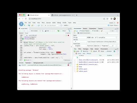
setwd("~/data/RNAseq") ## RNAseq is the folder where saved the salmon_quant and kallisto_quant
(salmon_files <- dir("salmon_quant", "sf$", 
                     recursive = TRUE, 
                     full.names = TRUE))

txi.salmon <- tximport(salmon_files, type = "salmon", 
                       tx2gene = t2g, ignoreTxVersion=TRUE)

sampleTable <- data.frame(condition = sub(".rep.", "", 
                                          basename(dirname(salmon_files))))
rownames(sampleTable) <- colnames(txi.salmon$counts)
dds.salmon <- DESeqDataSetFromTximport(txi.salmon, sampleTable, ~condition)
dds.salmon <- DESeq(dds.salmon)
res.salmon <- results(dds.salmon)
res.salmon[!is.na(res.salmon$padj), ]

run tximport + DESeq2 for kallisto results

(kallisto_files <- dir("kallisto_quant", "abundance.tsv", 
                       recursive = TRUE, full.names = TRUE))

txi.kallisto <- tximport(kallisto_files, type = "kallisto", 
                         tx2gene = t2g, ignoreTxVersion=TRUE)

sampleTable <- data.frame(condition = sub(".rep.", "", 
                                          basename(dirname(kallisto_files))))
rownames(sampleTable) <- colnames(txi.kallisto$counts)
dds.kallisto <- DESeqDataSetFromTximport(txi.kallisto, 
                                         sampleTable, ~condition)
dds.kallisto <- DESeq(dds.kallisto)
res.kallisto <- results(dds.kallisto)
res.kallisto[!is.na(res.kallisto$padj), ]

run Sleuth

The following code is showing how to use sleuth to do DE analysis. However, the sleuth package is not updated. It may be broken.

#BiocManager::install("pachterlab/sleuth")
library(sleuth)
samples <- dir("kallisto_quant")
s2c <- data.frame(path=dir("kallisto_quant", full.names = TRUE), 
                  sample=samples, 
                  condition=sub(".rep.", "", samples))
s2c
so <- sleuth_prep(s2c, ~-1+condition, target_mapping = t2g)
so <- sleuth_fit(so)
## which_beta must be in the colname of design table.
so <- sleuth_wt(so, which_beta = "conditionAblated")
sleuth_live(so)

scripts for ChIPseq

prepare index file for bwa

Run following code in Terminal panel of rstudio.

The sample data is located at “/home/rstudio/ChIPseq” folder. It is zebrafish H3 ChIP-seq data.

We will map the reads by BWA (Burrows-Wheeler Aligner). Compare to Bowtie2, BWA is a little slower but a bit more accurate and provides information on which alignments are trustworthy. The bwa-mem mode is generally recommended for high-quality queries. It is not limited by sequence reads size as bwa-backtrack and bwa-sw. Aligning reads with bwa-mem, there are two steps, build the index and do alignment. BWA indexes the genome with an FM index based on the Burrows-Wheeler Transform to keep memory requirements low for the alignment process.

## change you working directory
mkdir -p $HOME/data/ChIPseq
ln -s $HOME/ChIPseq/fastq $HOME/data/ChIPseq/
cd $HOME/data/ChIPseq
## download the zebrafish GRCz11 genome from ENSEMBLE
wget ftp://ftp.ensembl.org/pub/release-105/fasta/danio_rerio/dna/Danio_rerio.GRCz11.dna.primary_assembly.fa.gz
## build the index
## -p: prefix for all index files
bwa index -p GRCz11 Danio_rerio.GRCz11.dna.primary_assembly.fa.gz

The data are only a subset of the whole genome. We will only use genes in chromosome 4, 13, 16 and 21 to speed up the test run.

# wget https://raw.githubusercontent.com/jianhong/genomictools/master/inst/extdata/Danio_rerio.GRCz11.dna.toy.fa.gz
ln -s /usr/local/lib/R/site-library/basicBioinformaticsDRC2024/extdata/Danio_rerio.GRCz11.dna.toy.fa.gz ./
## the following step will take about 3min
bwa index -p GRCz11.toy Danio_rerio.GRCz11.dna.toy.fa.gz

Run fastQC, mapping and MACS2

We will run the scripts in a bash loop. The samples are from two uninjured and two ablated fish heart tissue. We use fastQC to check the quality of raw reads. The results will saved to “fastqc” folder. You can go through the results by click the index.html file in each sub-folder. We will perform alignment on the single-end reads. For more information on BWA and its functionality please refer to the user manual. MACS2 will be used to call the peaks.

group=(Ablated Ablated Uninjured Uninjured)
tag=(Ablated.rep1 Ablated.rep2 Uninjured.rep1 Uninjured.rep2)
species=danRer11
prefix=bwa

for i in {0..3}
do
## fastQC
mkdir -p fastqc/${group[$i]}
fastqc -o fastqc/${group[$i]} -t 2 \
       fastq/${tag[$i]}.fastq.gz
## trim adapter, need trim_galore be installed, here we do not do this step
# mkdir -p fastq.trimmed
# trim_galore -q 15 --fastqc -o fastq.trimmed/${group[$i]} fastq/${tag[$i]}.fastq.gz

## mapping by bwa
mkdir -p sam
## -t: number of threads
## -M: mark shorter split hits as secondary, this is optional for Picard compatibility.
## >: save alignment to a SAM file
## 2>: save standard error to log file
bwa mem -M -t 2 GRCz11.toy \
           fastq/${tag[$i]}.fastq.gz \
           > sam/$prefix.$species.${tag[$i]}.sam \
           2> bwa.$prefix.$species.${tag[$i]}.log.txt

## convert sam file to bam and clean-up
mkdir -p bam
## -q: skip alignments with MAPQ samller than 30.
samtools view -bhS -q 30 sam/$prefix.$species.${tag[$i]}.sam > bam/$prefix.$species.${tag[$i]}.bam
rm sam/$prefix.$species.${tag[$i]}.sam
## sort and index the bam file for quick access.
samtools sort bam/$prefix.$species.${tag[$i]}.bam -o bam/$prefix.$species.${tag[$i]}.srt.bam
samtools index bam/$prefix.$species.${tag[$i]}.srt.bam
## remove un-sorted bam file.
rm bam/$prefix.$species.${tag[$i]}.bam

## we remove the duplicated by picard::MarkDuplicates. 
mkdir -p bam/picard
picard MarkDuplicates \
       INPUT=bam/$prefix.$species.${tag[$i]}.srt.bam \
       OUTPUT=bam/$prefix.$species.${tag[$i]}.srt.markDup.bam \
       METRICS_FILE=bam/picard/$prefix.$species.${tag[$i]}.srt.fil.picard_info.txt \
       REMOVE_DUPLICATES=true ASSUME_SORTED=true VALIDATION_STRINGENCY=LENIENT
samtools index bam/$prefix.$species.${tag[$i]}.srt.markDup.bam

## use deeptools::bamCoverage to generate bigwig files
## the bw file can be viewed in IGV
mkdir -p bw
bamCoverage -b bam/$prefix.$species.${tag[$i]}.srt.markDup.bam -o bw/$prefix.$species.${tag[$i]}.bw --normalizeUsing CPM

## call peaks by macs2
mkdir -p macs3/${tag[$i]}
## -g: mappable genome size
## -q: use minimum FDR 0.05 cutoff to call significant regions.
## -B: ask MACS3 to output bedGraph files for experiment.
## --nomodel --extsize 150: the subset data is not big enough (<1000 peak) for
## macs3 to generate a model. We manually feed one.
## because we used toy genome, the genome size we set as 10M
macs3 callpeak -t bam/${prefix}.$species.${tag[$i]}.srt.markDup.bam \
               -f BAM -g 10e6 -n ${prefix}.$species.${tag[$i]} \
               --outdir macs3/${tag[$i]} -q 0.05 \
               -B --nomodel --extsize 150

done

Differential analysis

We will use DiffBind package to do the differential analysis.

setwd("/home/rstudio/data/ChIPseq")
library("DiffBind")
(bams <- dir("bam", "markDup.bam$", full.names = TRUE))
(Peaks <- dir("macs3", "narrowPeak$", full.names = TRUE, recursive = TRUE))
(SampleID <- basename(dirname(Peaks)))
(Condition <- sub(".rep.", "", SampleID))
(Replicate <- sub("^.*rep", "", SampleID))
Peakcaller <- "macs3"
PeakFormat <- "narrowPeak"
samples <- data.frame(SampleID=SampleID,
                      Condition=Condition,
                      Replicate=Replicate,
                      bamReads=bams,
                      Peaks=Peaks,
                      Peakcaller=Peakcaller,
                      PeakFormat=PeakFormat,
                      ScoreCol=5)

pf <- "DiffBind"
out <- "sample.csv"
dir.create(pf)
write.csv(samples, file.path(pf, out))
chip <- dba(sampleSheet = file.path(pf, out))
pdf(file.path(pf, "DiffBind.sample.correlation.pdf"), width = 9, height = 9)
plot(chip)
dev.off()
pdf(file.path(pf, "DiffBind.PCA.plot.pdf"))
dba.plotPCA(chip, DBA_CONDITION, label=DBA_ID)
dev.off()

chip <- dba.count(chip)
chip <- dba.normalize(chip) ## add for DiffBind 3.0
BLACKLIST <- FALSE ## fish data, no blacklist yet.
chip <- dba.blacklist(chip, blacklist=BLACKLIST, greylist=FALSE)
chip <- dba.contrast(chip, minMembers=2, categories = DBA_CONDITION)
chip <- dba.analyze(chip, bBlacklist = FALSE, bGreylist = FALSE)
chip.DB <- dba.report(chip, th=1)
head(chip.DB)
write.csv(chip.DB, file.path(pf, "DiffBind.results.csv"), row.names=FALSE)

Jianhong Ou

Learning Objectives:

Set-up

Install docker

Run kallisto and Salmon for RNA-seq

R scripts for RNAseq

prepare the transcripts to genes map table

run tximport + DESeq2 for Salmon results

run tximport + DESeq2 for kallisto results

run Sleuth

scripts for ChIPseq

prepare index file for bwa

Run fastQC, mapping and MACS2

Differential analysis