Four steps for peak annotation
The functions, toGRanges, annotatePeakInBatch, and addGeneIDs in the ChIPpeakAnno, make the annotation of ChIP-Seq peaks streamlined into four major steps:
Read peak data with
toGRangesGenerate annotation data with
toGRangesAnnotate peaks with
annotatePeakInBatchAdd additional informations with
addGeneIDs
## First, load the ChIPpeakAnno package
library(ChIPpeakAnno)
Step 1: convert the peak data from bed/broadPeak/narrowPeak etc. to GRanges with the toGRanges method
Here we use broadPeak file format as example.
## the sample file is included in ChIPpeakAnno package.
## chage the file path into your own file path to handle your data
path <- system.file("extdata", "Tead4.broadPeak", package="ChIPpeakAnno")
## toGRanges is overlaoded method,
## by define the correct file format to import the file in correct coordinates
peaks <- toGRanges(path, format="broadPeak")
## see top 2 lines of the imported peaks.
## the imported peaks will be packaged into GRanges object
head(peaks, n=2)
## GRanges object with 2 ranges and 4 metadata columns:
##             seqnames        ranges strand |     score signalValue    pValue
##                <Rle>     <IRanges>  <Rle> | <integer>   <numeric> <numeric>
##   peak12338     chr2 175473-176697      * |       206      668.42        -1
##   peak12339     chr2 246412-246950      * |        31      100.23        -1
##                qValue
##             <numeric>
##   peak12338        -1
##   peak12339        -1
##   -------
##   seqinfo: 1 sequence from an unspecified genome; no seqlengths
Step 2: prepare annotation data with the toGRanges method
ChIP-seq is a kind of DNA-seq. In the mapping step, no transcriptome is used. In the annotation step, both Ensembl or UCSC annotations can be used. Depend on your research, less complex genome annotations, such as UCSC annotations, are prefearable for reproducible and robust gene/transcripts annotation. To discover and explain unknown biological mechanisms, more comprehensive and complex genome annotations are necessary, such as Ensembl.
Here we show how to prepare annotations based on TxDb package with the toGRanges method.
library(TxDb.Hsapiens.UCSC.hg19.knownGene)
annoDataTxDb <- toGRanges(TxDb.Hsapiens.UCSC.hg19.knownGene)
head(annoDataTxDb, n=2)
## GRanges object with 2 ranges and 0 metadata columns:
##      seqnames            ranges strand
##         <Rle>         <IRanges>  <Rle>
##    1    chr19 58858172-58874214      -
##   10     chr8 18248755-18258723      +
##   -------
##   seqinfo: 93 sequences (1 circular) from hg19 genome
We can also prepare annotations based on EnsDb package with the toGRanges method.
library(EnsDb.Hsapiens.v75) ##GRCh37.p13
annoDataEnsDb <- toGRanges(EnsDb.Hsapiens.v75)
head(annoDataEnsDb, n=2)
## GRanges object with 2 ranges and 1 metadata column:
##                   seqnames      ranges strand |   gene_name
##                      <Rle>   <IRanges>  <Rle> | <character>
##   ENSG00000223972     chr1 11869-14412      + |     DDX11L1
##   ENSG00000227232     chr1 14363-29806      - |      WASH7P
##   -------
##   seqinfo: 273 sequences from 2 genomes (hg19, GRCh37)
The shortage of offline annotation packages is that it may not contain up-to-date data. We can also use online annotation data via the biomaRt or AnnotationHub packages. However, to use the biomaRt package, you must be very clear that the default mart service is based the newrest genome assembly. For example, if you are annotating the data mapped to hg19/GRCh37 or mm9/NCBIM37 assembly, you must change the default server into achive server. For more details, please refer the documentation of the biomaRt package.
library(biomaRt)
## here we use ensembl GRCh37.p13 (V75) service,
## use listEnsemblArchives() function to list the available host
## use listDatasets() function to list the available dataset
mart <- useMart(biomart = "ensembl", dataset = "hsapiens_gene_ensembl",
                host = "feb2014.archive.ensembl.org")
## use the getAnnotation function to obtain the TSS for ensembl GRCh37.p13.
annoDataMart <- getAnnotation(mart, featureType = "TSS")
annoDataMart[head(names(annoDataEnsDb), n=2)]
Here I show some sample code to get annotations from AnnotationHub.
library(AnnotationHub)
ah <- AnnotationHub()
hg19 <- AnnotationHub::query(ah, c("UCSC", "Hsapiens", "hg19", "knownGene"))
hg19
## AnnotationHub with 1 record
## # snapshotDate(): 2020-07-20
## # names(): AH52258
## # $dataprovider: UCSC
## # $species: Homo sapiens
## # $rdataclass: TxDb
## # $rdatadateadded: 2016-12-22
## # $title: TxDb.Hsapiens.UCSC.hg19.knownGene.sqlite
## # $description: UCSC transcript based annotations for Homo sapiens
## # $taxonomyid: 9606
## # $genome: UCSC genomes
## # $sourcetype: FASTA
## # $sourceurl: http://genome.ucsc.edu/, http://hgdownload.cse.ucsc.edu/golden...
## # $sourcesize: NA
## # $tags: c("UCSC", "Transcript", "Annotation")
## # retrieve record with 'object[["AH52258"]]'
hg19TxDb <- hg19[["AH52258"]] annoDataHg19<- toGRanges(hg19TxDb) identical(annoDataHg19, annoDataTxDb)
## [1] TRUE## retrieve the gencode v32 annotation GRCh37 <- AnnotationHub::query(ah, c("GRCh37", "GENCODE", "v32", "TxDb")) annoDataGencode <- toGRanges(GRCh37[["AH75188"]]) head(annoDataGencode, n=2)
## GRanges object with 2 ranges and 0 metadata columns:
##                        seqnames            ranges strand
##                           <Rle>         <IRanges>  <Rle>
##   ENSG00000000003.15_3     chrX 99882105-99894988      -
##    ENSG00000000005.6_3     chrX 99839933-99854882      +
##   -------
##   seqinfo: 25 sequences (1 circular) from hg19 genome
Step 3: annotate the peaks with the annotatePeakInBatch function.
Here we will compare the difference among differnt annotation sources.
First we compare the annotations from ensembl GRCh37.p13 between the EnsDb.Hsapiens.v75 package and ensembl archives.
seqlevelsStyle(annoDataEnsDb)
## [1] "UCSC" "NCBI"seqlevelsStyle(peaks)
## [1] "UCSC"## keep the seqnames in the same style if(!identical(seqlevelsStyle(peaks), seqlevelsStyle(annoDataEnsDb))){ seqlevelsStyle(peaks) <- seqlevelsStyle(annoDataEnsDb)[1] } ## do annotation by nearest TSS of Ensembl GRCh37.p13 annoEnsDb <- annotatePeakInBatch(peaks, AnnotationData=annoDataEnsDb) head(annoEnsDb, n=2)
## GRanges object with 2 ranges and 13 metadata columns:
##                             seqnames        ranges strand |     score
##                                <Rle>     <IRanges>  <Rle> | <integer>
##   peak12338.ENSG00000227061     chr2 175473-176697      * |       206
##   peak12339.ENSG00000143727     chr2 246412-246950      * |        31
##                             signalValue    pValue    qValue        peak
##                               <numeric> <numeric> <numeric> <character>
##   peak12338.ENSG00000227061      668.42        -1        -1   peak12338
##   peak12339.ENSG00000143727      100.23        -1        -1   peak12339
##                                     feature start_position end_position
##                                 <character>      <integer>    <integer>
##   peak12338.ENSG00000227061 ENSG00000227061         197569       202605
##   peak12339.ENSG00000143727 ENSG00000143727         264140       278283
##                             feature_strand insideFeature distancetoFeature
##                                <character>   <character>         <numeric>
##   peak12338.ENSG00000227061              +      upstream            -22096
##   peak12339.ENSG00000143727              +      upstream            -17728
##                             shortestDistance fromOverlappingOrNearest
##                                    <integer>              <character>
##   peak12338.ENSG00000227061            20872          NearestLocation
##   peak12339.ENSG00000143727            17190          NearestLocation
##   -------
##   seqinfo: 1 sequence from an unspecified genome; no seqlengths
# A pie chart can be used to demonstrate the overlap features of the peaks. pie1(table(annoEnsDb$insideFeature))
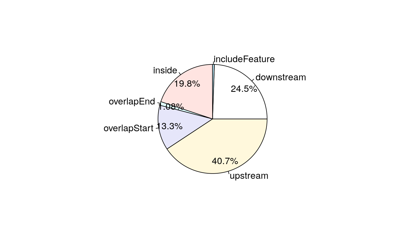
Pie chart of common peaks among EnsDb features.
## keep the seqnames in the same style
if(!identical(seqlevelsStyle(peaks), seqlevelsStyle(annoDataMart))){
  seqlevelsStyle(peaks) <- seqlevelsStyle(annoDataMart)[1]
}
## do annotation by nearest TSS of Ensembl GRCh37.p13
annoMart <- annotatePeakInBatch(peaks, AnnotationData=annoDataMart)
head(annoMart, n=2)
## GRanges object with 2 ranges and 13 metadata columns:
##                             seqnames        ranges strand |     score
##                                <Rle>     <IRanges>  <Rle> | <integer>
##   peak12338.ENSG00000227061     chr2 175473-176697      * |       206
##   peak12339.ENSG00000143727     chr2 246412-246950      * |        31
##                             signalValue    pValue    qValue        peak
##                               <numeric> <numeric> <numeric> <character>
##   peak12338.ENSG00000227061      668.42        -1        -1   peak12338
##   peak12339.ENSG00000143727      100.23        -1        -1   peak12339
##                                     feature start_position end_position
##                                 <character>      <integer>    <integer>
##   peak12338.ENSG00000227061 ENSG00000227061         197569       202605
##   peak12339.ENSG00000143727 ENSG00000143727         264140       278283
##                             feature_strand insideFeature distancetoFeature
##                                <character>   <character>         <numeric>
##   peak12338.ENSG00000227061              +      upstream            -22096
##   peak12339.ENSG00000143727              +      upstream            -17728
##                             shortestDistance fromOverlappingOrNearest
##                                    <integer>              <character>
##   peak12338.ENSG00000227061            20872          NearestLocation
##   peak12339.ENSG00000143727            17190          NearestLocation
##   -------
##   seqinfo: 1 sequence from an unspecified genome; no seqlengths
# A pie chart can be used to demonstrate the overlap features of the peaks. pie1(table(annoMart$insideFeature))

Pie chart of common peaks among biomart features.
We can see the minor difference between them. Lets check the reasons.
## check how many annotations are different from each other
table(start(annoDataMart[names(annoDataEnsDb)])==start(annoDataEnsDb))
##
## FALSE  TRUE
## 417 63685##
## FALSE TRUE
## 417 63685## get the samples head(annoDataMart[names(annoDataEnsDb)][ start(annoDataMart[names(annoDataEnsDb)])!=start(annoDataEnsDb)], n=2)
## GRanges object with 2 ranges and 1 metadata column:
##           seqnames      ranges strand |            description
##              <Rle>   <IRanges>  <Rle> |            <character>
##   LRG_198  LRG_198  5001-40990      + | agrin [Source:HGNC S..
##   LRG_262  LRG_262 33310-58918      + | pleckstrin homology ..
##   -------
## seqinfo: 690 sequences from an unspecified genome; no seqlengths## GRanges object with 2 ranges and 1 metadata column:
## seqnames ranges strand | gene_name
## <Rle> <IRanges> <Rle> | <character>
## LRG_198 chr1 955503-991492 + | LRG_198
## LRG_262 chr1 6526152-6551760 - | LRG_262
## -------
## seqinfo: 273 sequences from 2 genomes (hg19, GRCh37)## check the biomart output getBM(attributes = c("ensembl_gene_id", 'chromosome_name', "description"), filters = "ensembl_gene_id", values = c("LRG_198", "LRG_262"), mart = mart)
##   ensembl_gene_id chromosome_name
## 1         LRG_198         LRG_198
## 2         LRG_262         LRG_262
##                                                                                                    description
## 1                                                                           agrin [Source:HGNC Symbol;Acc:329]
## 2 pleckstrin homology domain containing, family G (with RhoGef domain) member 5 [Source:HGNC Symbol;Acc:29105]
Here we can see that the EnsDb.Hsapiens.v75 package already fixed the issue of chromosome_name issue, where the biomart online still output the wrong chromosome_name.
Now we annotate the peaks by UCSC hg19 annotations.
## keep the seqnames in the same style
if(!identical(seqlevelsStyle(peaks), seqlevelsStyle(annoDataTxDb))){
  seqlevelsStyle(peaks) <- seqlevelsStyle(annoDataTxDb)[1]
}
## do annotation by nearest TSS of UCSC hg19 annotations
annoTxDb <- annotatePeakInBatch(peaks, AnnotationData=annoDataTxDb)
head(annoTxDb, n=2)
## GRanges object with 2 ranges and 13 metadata columns:
##                   seqnames        ranges strand |     score signalValue
##                      <Rle>     <IRanges>  <Rle> | <integer>   <numeric>
##   peak12338.26751     chr2 175473-176697      * |       206      668.42
##   peak12339.26751     chr2 246412-246950      * |        31      100.23
##                      pValue    qValue        peak     feature start_position
##                   <numeric> <numeric> <character> <character>      <integer>
##   peak12338.26751        -1        -1   peak12338       26751         218136
##   peak12339.26751        -1        -1   peak12339       26751         218136
##                   end_position feature_strand insideFeature distancetoFeature
##                      <integer>    <character>   <character>         <numeric>
##   peak12338.26751       264810              -    downstream             89337
##   peak12339.26751       264810              -        inside             18398
##                   shortestDistance fromOverlappingOrNearest
##                          <integer>              <character>
##   peak12338.26751            41439          NearestLocation
##   peak12339.26751            17860          NearestLocation
##   -------
##   seqinfo: 1 sequence from an unspecified genome; no seqlengths
# A pie chart can be used to demonstrate the overlap features of the peaks. pie1(table(annoTxDb$insideFeature))
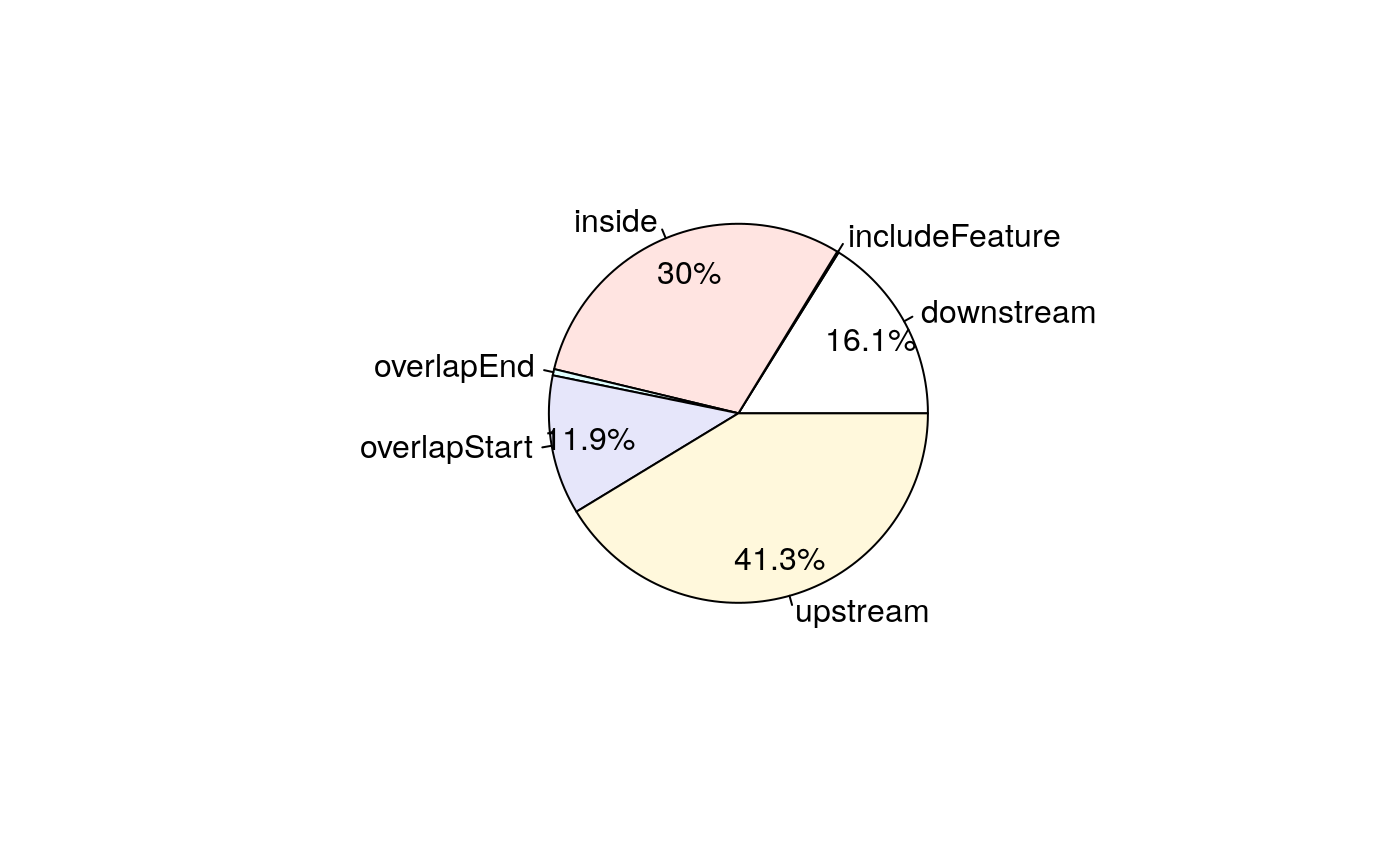
Pie chart of common peaks among TxDb features.
Now we try to use gencode v32 annotations to annotate the peaks.
## keep the seqnames in the same style
if(!identical(seqlevelsStyle(peaks), seqlevelsStyle(annoDataGencode))){
  seqlevelsStyle(peaks) <- seqlevelsStyle(annoDataGencode)[1]
}
## do annotation by nearest TSS of Gencode
annoGencode <- annotatePeakInBatch(peaks, AnnotationData=annoDataGencode)
head(annoGencode, n=2)
## GRanges object with 2 ranges and 13 metadata columns:
##                                  seqnames        ranges strand |     score
##                                     <Rle>     <IRanges>  <Rle> | <integer>
##    peak12338.ENSG00000227061.2_6     chr2 175473-176697      * |       206
##   peak12339.ENSG00000143727.16_3     chr2 246412-246950      * |        31
##                                  signalValue    pValue    qValue        peak
##                                    <numeric> <numeric> <numeric> <character>
##    peak12338.ENSG00000227061.2_6      668.42        -1        -1   peak12338
##   peak12339.ENSG00000143727.16_3      100.23        -1        -1   peak12339
##                                               feature start_position
##                                           <character>      <integer>
##    peak12338.ENSG00000227061.2_6  ENSG00000227061.2_6         197569
##   peak12339.ENSG00000143727.16_3 ENSG00000143727.16_3         264140
##                                  end_position feature_strand insideFeature
##                                     <integer>    <character>   <character>
##    peak12338.ENSG00000227061.2_6       209892              +      upstream
##   peak12339.ENSG00000143727.16_3       278283              +      upstream
##                                  distancetoFeature shortestDistance
##                                          <numeric>        <integer>
##    peak12338.ENSG00000227061.2_6            -22096            20872
##   peak12339.ENSG00000143727.16_3            -17728            17190
##                                  fromOverlappingOrNearest
##                                               <character>
##    peak12338.ENSG00000227061.2_6          NearestLocation
##   peak12339.ENSG00000143727.16_3          NearestLocation
##   -------
##   seqinfo: 1 sequence from an unspecified genome; no seqlengths
# A pie chart can be used to demonstrate the overlap features of the peaks. pie1(table(annoGencode$insideFeature))
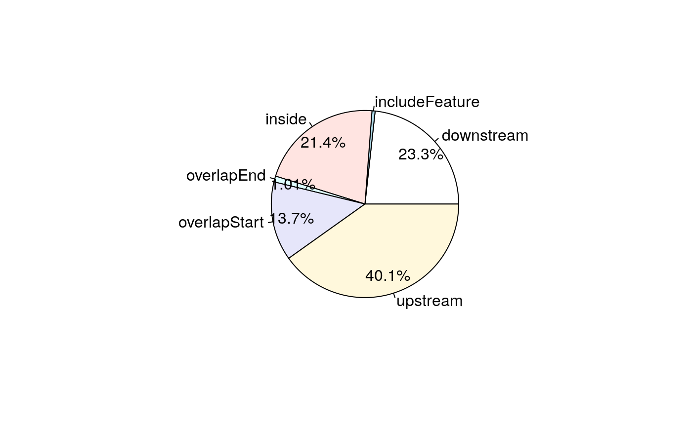
Pie chart of common peaks among Gencode features.
We can see the difference between the annotations among Ensembl, UCSC and Gencode in annotation. Let’s check the overlaps of annotations.
Ensembl <- unique(annoDataEnsDb)
UCSC <- unique(annoDataTxDb)
Gencode <- unique(annoDataGencode)
## make the sequence info to same, otherwise can not compare.
genome(seqinfo(Gencode)) <-
  genome(seqinfo(UCSC)) <-
  genome(seqinfo(Ensembl)) <- factor("hg19")
isCircular(seqinfo(UCSC)) <- rep(FALSE, length(seqlevels(UCSC)))
isCircular(seqinfo(Gencode)) <- rep(FALSE, length(seqlevels(Gencode)))
seqlevels(Ensembl) <- sub("chrMT", "chrM", seqlevels(Ensembl))
seqlengths(Ensembl)["chrM"] <- seqlengths(UCSC)["chrM"]
## find the overlaps by max gap = 0 bp.
ol <- findOverlapsOfPeaks(Ensembl,
                          UCSC,
                          Gencode,
                          ignore.strand = FALSE,
                          connectedPeaks="keepAll")
## venn diagram to show the overlaps
makeVennDiagram(ol, connectedPeaks = "keepAll")
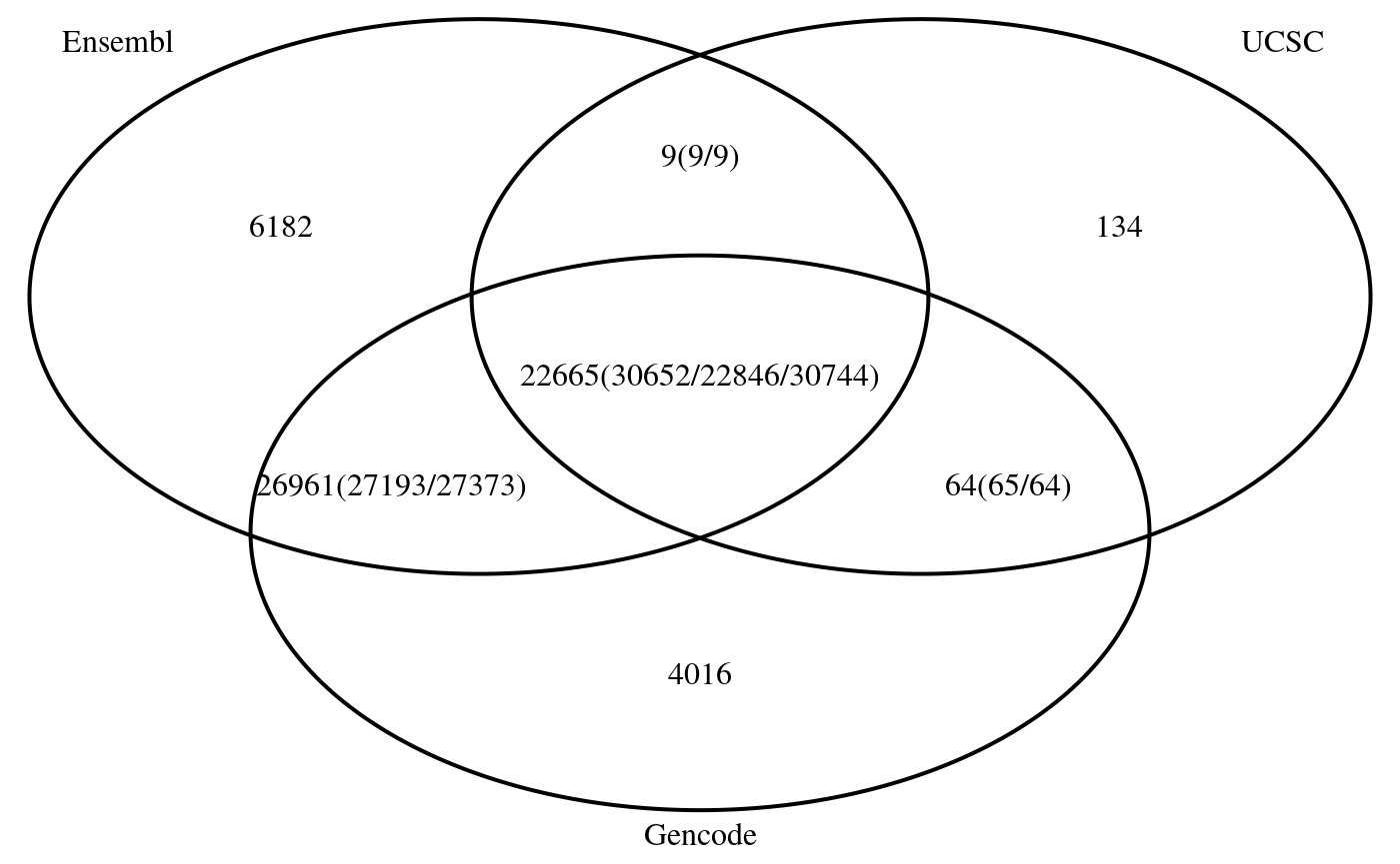
The overlap and intersection among UCSC, Ensembl, and Gencode annotations.
## $p.value
##      Ensembl UCSC Gencode pval
## [1,]       0    1       1  NaN
## [2,]       1    0       1  NaN
## [3,]       1    1       0  NaN
##
## $vennCounts
##      Ensembl UCSC Gencode Counts count.Ensembl count.UCSC count.Gencode
## [1,]       0    0       0      0             0          0             0
## [2,]       0    0       1   4016             0          0          4016
## [3,]       0    1       0    134             0        134             0
## [4,]       0    1       1     64             0         65            64
## [5,]       1    0       0   6182          6182          0             0
## [6,]       1    0       1  26961         27193          0         27373
## [7,]       1    1       0      9             9          9             0
## [8,]       1    1       1  22665         30652      22846         30744
## attr(,"class")
## [1] "VennCounts"
Step 4: add additional annotation with the addGeneIDs function
library(org.Hs.eg.db)
annoEnsDb <- addGeneIDs(annoEnsDb, orgAnn="org.Hs.eg.db",
                        feature_id_type="ensembl_gene_id",
                        IDs2Add=c("symbol"))
head(annoEnsDb, n=2)
## GRanges object with 2 ranges and 14 metadata columns:
##                             seqnames        ranges strand |     score
##                                <Rle>     <IRanges>  <Rle> | <integer>
##   peak12338.ENSG00000227061     chr2 175473-176697      * |       206
##   peak12339.ENSG00000143727     chr2 246412-246950      * |        31
##                             signalValue    pValue    qValue        peak
##                               <numeric> <numeric> <numeric> <character>
##   peak12338.ENSG00000227061      668.42        -1        -1   peak12338
##   peak12339.ENSG00000143727      100.23        -1        -1   peak12339
##                                     feature start_position end_position
##                                 <character>      <integer>    <integer>
##   peak12338.ENSG00000227061 ENSG00000227061         197569       202605
##   peak12339.ENSG00000143727 ENSG00000143727         264140       278283
##                             feature_strand insideFeature distancetoFeature
##                                <character>   <character>         <numeric>
##   peak12338.ENSG00000227061              +      upstream            -22096
##   peak12339.ENSG00000143727              +      upstream            -17728
##                             shortestDistance fromOverlappingOrNearest
##                                    <integer>              <character>
##   peak12338.ENSG00000227061            20872          NearestLocation
##   peak12339.ENSG00000143727            17190          NearestLocation
##                                  symbol
##                             <character>
##   peak12338.ENSG00000227061        <NA>
##   peak12339.ENSG00000143727        ACP1
##   -------
##   seqinfo: 1 sequence from an unspecified genome; no seqlengths
annoTxDb <- addGeneIDs(annoTxDb, orgAnn="org.Hs.eg.db", feature_id_type="entrez_id", IDs2Add=c("symbol")) head(annoTxDb, n=2)
## GRanges object with 2 ranges and 14 metadata columns:
##                   seqnames        ranges strand |     score signalValue
##                      <Rle>     <IRanges>  <Rle> | <integer>   <numeric>
##   peak12338.26751     chr2 175473-176697      * |       206      668.42
##   peak12339.26751     chr2 246412-246950      * |        31      100.23
##                      pValue    qValue        peak     feature start_position
##                   <numeric> <numeric> <character> <character>      <integer>
##   peak12338.26751        -1        -1   peak12338       26751         218136
##   peak12339.26751        -1        -1   peak12339       26751         218136
##                   end_position feature_strand insideFeature distancetoFeature
##                      <integer>    <character>   <character>         <numeric>
##   peak12338.26751       264810              -    downstream             89337
##   peak12339.26751       264810              -        inside             18398
##                   shortestDistance fromOverlappingOrNearest      symbol
##                          <integer>              <character> <character>
##   peak12338.26751            41439          NearestLocation      SH3YL1
##   peak12339.26751            17860          NearestLocation      SH3YL1
##   -------
## seqinfo: 1 sequence from an unspecified genome; no seqlengthsannoGencode$entrez_id <- xget(sub("(ENSG\\d{11}).*$", "\\1", as.character(annoGencode$feature)), org.Hs.egENSEMBL2EG, output = "last") annoGencode$symbol[!is.na(annoGencode$entrez_id)] <- xget(annoGencode$entrez_id[!is.na(annoGencode$entrez_id)], org.Hs.egSYMBOL) head(annoGencode)
## GRanges object with 6 ranges and 15 metadata columns:
##                                  seqnames        ranges strand |     score
##                                     <Rle>     <IRanges>  <Rle> | <integer>
##    peak12338.ENSG00000227061.2_6     chr2 175473-176697      * |       206
##   peak12339.ENSG00000143727.16_3     chr2 246412-246950      * |        31
##   peak12340.ENSG00000143727.16_3     chr2 249352-250233      * |       195
##   peak12341.ENSG00000143727.16_3     chr2 259896-261404      * |       510
##   peak12342.ENSG00000143727.16_3     chr2 261931-263148      * |        48
##    peak12343.ENSG00000236856.1_6     chr2 378232-378871      * |       132
##                                  signalValue    pValue    qValue        peak
##                                    <numeric> <numeric> <numeric> <character>
##    peak12338.ENSG00000227061.2_6      668.42        -1        -1   peak12338
##   peak12339.ENSG00000143727.16_3      100.23        -1        -1   peak12339
##   peak12340.ENSG00000143727.16_3      630.65        -1        -1   peak12340
##   peak12341.ENSG00000143727.16_3     1649.19        -1        -1   peak12341
##   peak12342.ENSG00000143727.16_3      155.56        -1        -1   peak12342
##    peak12343.ENSG00000236856.1_6      426.52        -1        -1   peak12343
##                                               feature start_position
##                                           <character>      <integer>
##    peak12338.ENSG00000227061.2_6  ENSG00000227061.2_6         197569
##   peak12339.ENSG00000143727.16_3 ENSG00000143727.16_3         264140
##   peak12340.ENSG00000143727.16_3 ENSG00000143727.16_3         264140
##   peak12341.ENSG00000143727.16_3 ENSG00000143727.16_3         264140
##   peak12342.ENSG00000143727.16_3 ENSG00000143727.16_3         264140
##    peak12343.ENSG00000236856.1_6  ENSG00000236856.1_6         388412
##                                  end_position feature_strand insideFeature
##                                     <integer>    <character>   <character>
##    peak12338.ENSG00000227061.2_6       209892              +      upstream
##   peak12339.ENSG00000143727.16_3       278283              +      upstream
##   peak12340.ENSG00000143727.16_3       278283              +      upstream
##   peak12341.ENSG00000143727.16_3       278283              +      upstream
##   peak12342.ENSG00000143727.16_3       278283              +      upstream
##    peak12343.ENSG00000236856.1_6       416885              +      upstream
##                                  distancetoFeature shortestDistance
##                                          <numeric>        <integer>
##    peak12338.ENSG00000227061.2_6            -22096            20872
##   peak12339.ENSG00000143727.16_3            -17728            17190
##   peak12340.ENSG00000143727.16_3            -14788            13907
##   peak12341.ENSG00000143727.16_3             -4244             2736
##   peak12342.ENSG00000143727.16_3             -2209              992
##    peak12343.ENSG00000236856.1_6            -10180             9541
##                                  fromOverlappingOrNearest   entrez_id
##                                               <character> <character>
##    peak12338.ENSG00000227061.2_6          NearestLocation        <NA>
##   peak12339.ENSG00000143727.16_3          NearestLocation          52
##   peak12340.ENSG00000143727.16_3          NearestLocation          52
##   peak12341.ENSG00000143727.16_3          NearestLocation          52
##   peak12342.ENSG00000143727.16_3          NearestLocation          52
##    peak12343.ENSG00000236856.1_6          NearestLocation        <NA>
##                                       symbol
##                                  <character>
##    peak12338.ENSG00000227061.2_6        <NA>
##   peak12339.ENSG00000143727.16_3        ACP1
##   peak12340.ENSG00000143727.16_3        ACP1
##   peak12341.ENSG00000143727.16_3        ACP1
##   peak12342.ENSG00000143727.16_3        ACP1
##    peak12343.ENSG00000236856.1_6        <NA>
##   -------
## seqinfo: 1 sequence from an unspecified genome; no seqlengthslibrary(UpSetR) upset(fromList(list(Ensembl=unique(annoEnsDb$symbol), UCSC=unique(annoTxDb$symbol), Gencode=unique(annoGencode$symbol))), order.by = "freq")
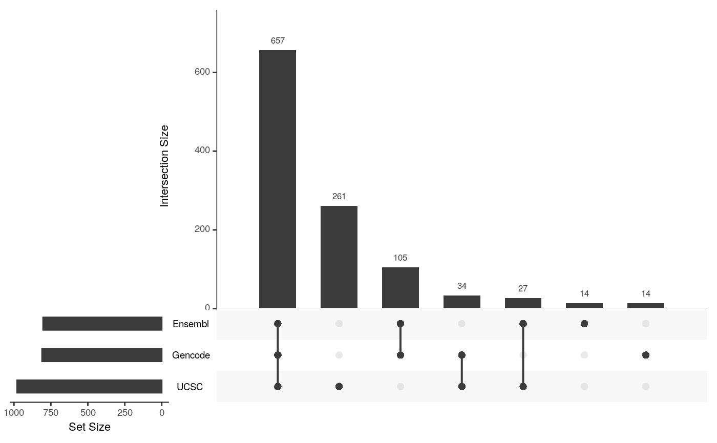
upset plot of common gene symbols among annotations by Ensembl, UCSC and Gencode features.
As a conclusion, annotate with different annotation resources, even the other parameter keep same, the annotations will be different from each other. To improve the reproducibility, accuracy of an annotation source should be provided. Some people were advertizing their tools by playing this trick by using different annotations to mislead users.
Find overlaps for replicates
The function findOverlapsOfPeaks returns an object of overlappingPeaks, which contains there elements: venn_cnt, peaklist (a list of
overlapping peaks or unique peaks), and overlappingPeaks (a list of data frame consists of the annotation of all the overlapping peaks).
The following examples illustrate the usage of this method to convert BED and GFF file to GRanges, add metadata from orignal peaks to the overlap GRanges using function addMetadata, and visualize the overlapping using function makeVennDiagram.
library(ChIPpeakAnno)
bed <- system.file("extdata", "MACS_output.bed", package="ChIPpeakAnno")
gr1 <- toGRanges(bed, format="BED", header=FALSE)
## one can also try import from rtracklayer
gff <- system.file("extdata", "GFF_peaks.gff", package="ChIPpeakAnno")
gr2 <- toGRanges(gff, format="GFF", header=FALSE, skip=3)
## must keep the class exactly same as gr1$score, i.e., numeric.
gr2$score <- as.numeric(gr2$score)
ol <- findOverlapsOfPeaks(gr1, gr2, connectedPeaks = "keepAll")
## add metadata (mean of score) to the overlapping peaks
ol <- addMetadata(ol, colNames="score", FUN=mean)
head(ol$peaklist[["gr1///gr2"]], n=2)
## GRanges object with 2 ranges and 2 metadata columns:
##       seqnames        ranges strand |                           peakNames
##          <Rle>     <IRanges>  <Rle> |                     <CharacterList>
##   [1]     chr1 713791-715578      * | gr1__MACS_peak_13,gr2__001,gr2__002
##   [2]     chr1 724851-727191      * |          gr2__003,gr1__MACS_peak_14
##           score
##       <numeric>
##   [1]   850.203
##   [2]    29.170
##   -------
## seqinfo: 1 sequence from an unspecified genome; no seqlengthsmakeVennDiagram(ol, fill=c("#009E73", "#F0E442"), # circle fill color col=c("#D55E00", "#0072B2"), #circle border color cat.col=c("#D55E00", "#0072B2")) # label color, keep same as circle border color

Venn diagram of overlaps for replicated experiments
## $p.value
##      gr1 gr2 pval
## [1,]   1   1    0
##
## $vennCounts
##      gr1 gr2 Counts count.gr1 count.gr2
## [1,]   0   0      0         0         0
## [2,]   0   1     61         0        61
## [3,]   1   0     62        62         0
## [4,]   1   1    166       168       169
## attr(,"class")
## [1] "VennCounts"
But if we check the sum of the overlaps, the total number for each sample are not identical to inputed peak number. This can be fixed by set ‘connectedPeaks’ parameter into ‘keepAll’.
length(gr1)
## [1] 230length(gr2)
## [1] 23062+166
## [1] 22861+166
## [1] 227makeVennDiagram(ol, fill=c("#009E73", "#F0E442"), col=c("#D55E00", "#0072B2"), cat.col=c("#D55E00", "#0072B2"), connectedPeaks = "keepAll")
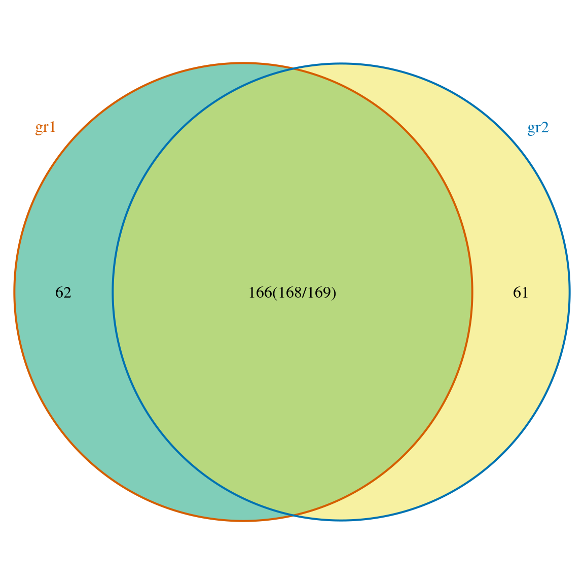
Venn diagram of overlaps with all original counts.
## $p.value
##      gr1 gr2 pval
## [1,]   1   1    0
##
## $vennCounts
##      gr1 gr2 Counts count.gr1 count.gr2
## [1,]   0   0      0         0         0
## [2,]   0   1     61         0        61
## [3,]   1   0     62        62         0
## [4,]   1   1    166       168       169
## attr(,"class")
## [1] "VennCounts"
Select annotation method
Visualize binding site distribution relative to features
The assignChromosomeRegion function can be used to summarize the distribution of peaks over different type of features such as exon, intron, enhancer, proximal promoter, 5’ UTR and 3’ UTR. This distribution can be summarized in peak centric or nucleotide centric view using the function assignChromosomeRegion. Please note that one peak might span multiple type of features, leading to the number of annotated features greater than the total number of input peaks. At the peak centric view, precedence will dictate the annotation order when peaks span multiple type of features.
The sample code here plots the distribution of peaks are enriched around the promoters.
overlaps <- ol$peaklist[["gr1///gr2"]] ## get the overlapping peaks
## load TxDb to assign genomic elements
library(TxDb.Hsapiens.UCSC.hg19.knownGene)
aCR<-assignChromosomeRegion(overlaps, nucleotideLevel=FALSE,
                           precedence=c("Promoters", "immediateDownstream",
                                         "fiveUTRs", "threeUTRs",
                                         "Exons", "Introns"),
                           TxDb=TxDb.Hsapiens.UCSC.hg19.knownGene)
barplot(aCR$percentage, las=3)
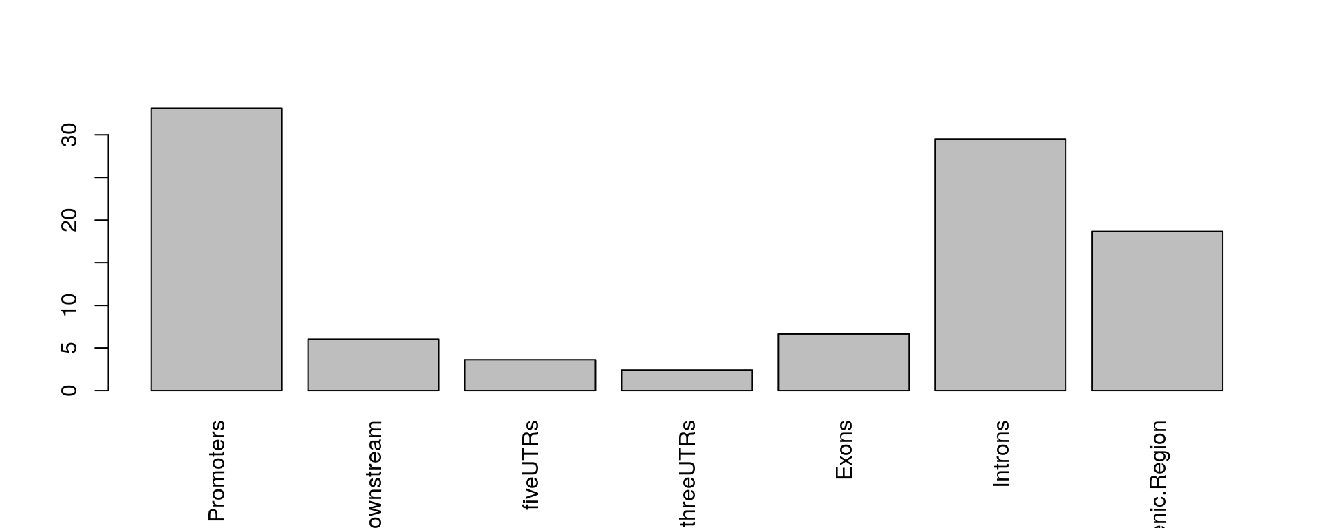
Peak distribution over different genomic features.
In addition, the distribution of the distance of overlapped peaks to the nearest feature such as the transcription start sites (TSS) can be plotted by the binOverFeature function. The sample code here plots the distribution of peaks around the TSS.
binOverFeature(overlaps, annotationData=annoDataTxDb,
               radius=5000, nbins=20, FUN=length, errFun=0,
               ylab="count",
               main="Distribution of aggregated peak numbers around TSS")
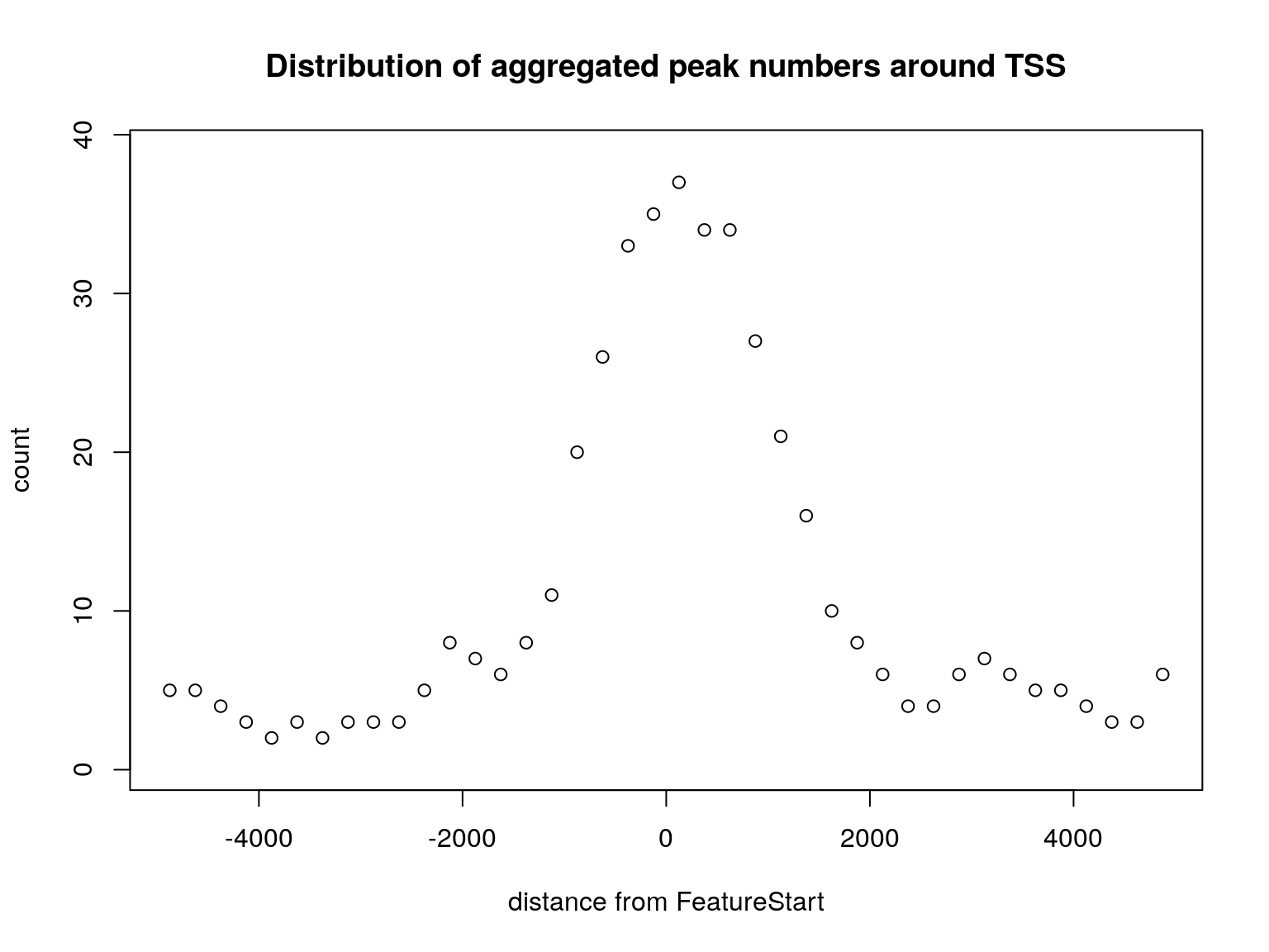
Distribution of peaks around transcript start sites.
Annotate peaks
The annotatePeakInBatch function provide multiple methods to annotate the peaks and those methods can be set by combination of multiple parameters. The ‘output’ is the key parameter to determine the annotation method. The default method is search the nearest features calculated as ‘PeakLoc - FeatureLocForDistance’. For more information, please refer the documentation of the annotatePeakInBatch function.
As shown from the distribution of aggregated peak numbers around TSS and the distribution of peaks in different of chromosome regions, most of the peaks locate around TSS. Therefore, it is reasonable to use the annotatePeakInBatch or annoPeaks to annotate the peaks to the promoter regions of Hg19/GRCh37 genes. Promoters can be specified with ‘bindingRegion’. For the following example, promoter region is defined as upstream 2000 and downstream 500 from TSS (bindingRegion=c(-2000, 500)).
overlaps.anno <- annotatePeakInBatch(overlaps,
                                     AnnotationData=annoDataTxDb,
                                     output="nearestBiDirectionalPromoters",
                                     bindingRegion=c(-2000, 500))
library(org.Hs.eg.db)
overlaps.anno <- addGeneIDs(overlaps.anno,
                            "org.Hs.eg.db",
                            feature_id_type="entrez_id",
                            IDs2Add = "symbol")
head(overlaps.anno, n=2)
## GRanges object with 2 ranges and 10 metadata columns:
##      seqnames        ranges strand |                           peakNames
##         <Rle>     <IRanges>  <Rle> |                     <CharacterList>
##   X1     chr1 713791-715578      * | gr1__MACS_peak_13,gr2__001,gr2__002
##   X4     chr1 856361-856999      * |          gr1__MACS_peak_17,gr2__005
##          score        peak     feature feature.ranges feature.strand  distance
##      <numeric> <character> <character>      <IRanges>          <Rle> <integer>
##   X1   850.203          X1   100288069  700245-714068              -         0
##   X4    54.690          X4   100130417  852953-854817              -      1543
##      insideFeature distanceToSite       symbol
##        <character>      <integer>  <character>
##   X1  overlapStart              0 LOC100288069
##   X4      upstream           1543    LINC02593
##   -------
## seqinfo: 1 sequence from an unspecified genome; no seqlengthslibrary(WriteXLS) WriteXLS(as.data.frame(unname(overlaps.anno)), "anno.xls")
The distribution of the common peaks around features can be visualized using a pie chart.
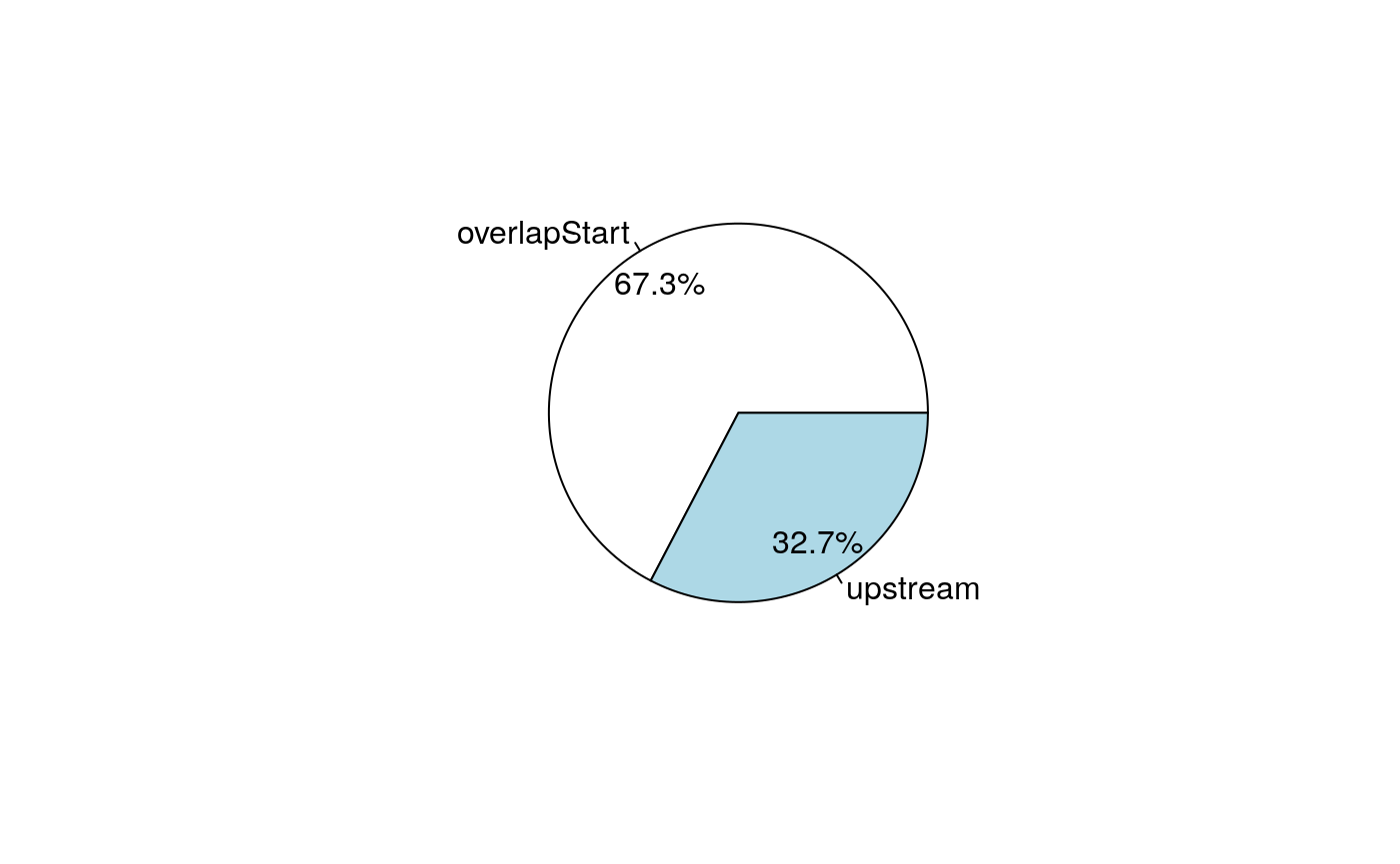
Pie chart of the distribution of common peaks around features.
Obtain enriched GO terms and Pathways
The following example shows how to use getEnrichedGO to obtain a list of enriched GO terms with annotated peaks. For pathway analysis, please use function getEnrichedPATH with reactome or KEGG database. Please note that by default feature_id_type is set as “ensembl_gene_id”. If you are using TxDb as annotation data, please set it to “entrez_id”.
over <- getEnrichedGO(overlaps.anno, orgAnn="org.Hs.eg.db",
                      feature_id_type="entrez_id",
                      maxP=.05, minGOterm=10,
                      multiAdjMethod="BH", condense=TRUE)
head(over[["bp"]][, -c(3, 10)], n=2)
## [1] go.id              go.term            Ontology           pvalue
## [5] count.InDataset    count.InGenome     totaltermInDataset totaltermInGenome
## [9] EntrezID
## <0 rows> (or 0-length row.names)library(reactome.db) path <- getEnrichedPATH(overlaps.anno, "org.Hs.eg.db", "reactome.db", feature_id_type="entrez_id", maxP=.05) head(path, n=2)
##        path.id EntrezID count.InDataset count.InGenome     pvalue
## 1 R-HSA-196849    55229               2            123 0.03029926
## 2 R-HSA-196849    65220               2            123 0.03029926
##   totaltermInDataset totaltermInGenome PATH
## 1                244            111075   NA
## 2                244            111075   NA
Output a summary of consensus in the peaks
There are multiple methods to get the consensus in the peaks:
output the fastq file by the
getAllPeakSequencefunction and search the motif by the 3rd program such as homer, MEME, and so on.test the pre-defined consensus patterns to see if target consensus are enriched or not by the
summarizePatternInPeaksfunction.calculate the z-scores of all combinations of oligonucleotide in a given length by Markove chain by the
oligoSummaryfunction.
Here is an example to get the Z-scores for short oligos.
library(seqinr)
library(BSgenome.Hsapiens.UCSC.hg19)
seq <- getAllPeakSequence(overlaps,
                          upstream=20, downstream=20,
                          genome=Hsapiens)
## output the fasta file for the 3nd program
write2FASTA(seq, "test.fa")
## summary of the short oligos
os <- oligoSummary(seq, oligoLength=6, MarkovOrder=3,
                   quickMotif=TRUE)
## plot the results
zscore <- sort(os$zscore)
h <- hist(zscore, breaks=100, main="Histogram of Z-score")
text(zscore[length(zscore)], max(h$counts)/10,
     labels=names(zscore[length(zscore)]), srt=90)
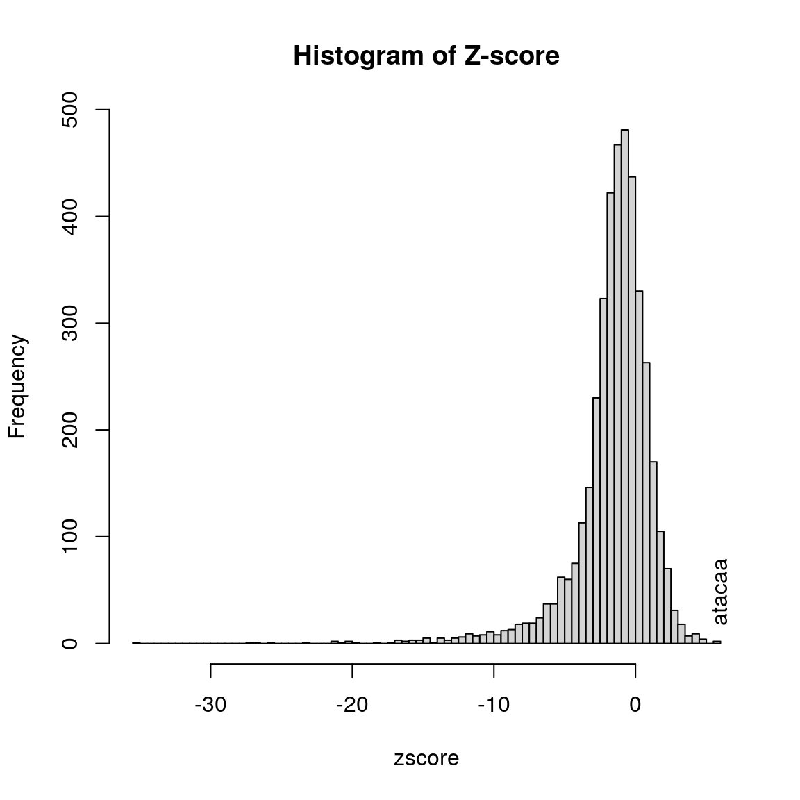
Histogram of Z-score of 6-mer
## generate the motifs
library(motifStack)
pfms <- mapply(function(.ele, id)
    new("pfm", mat=.ele, name=paste("SAMPLE motif", id)),
    os$motifs, 1:length(os$motifs))
motifStack(pfms)
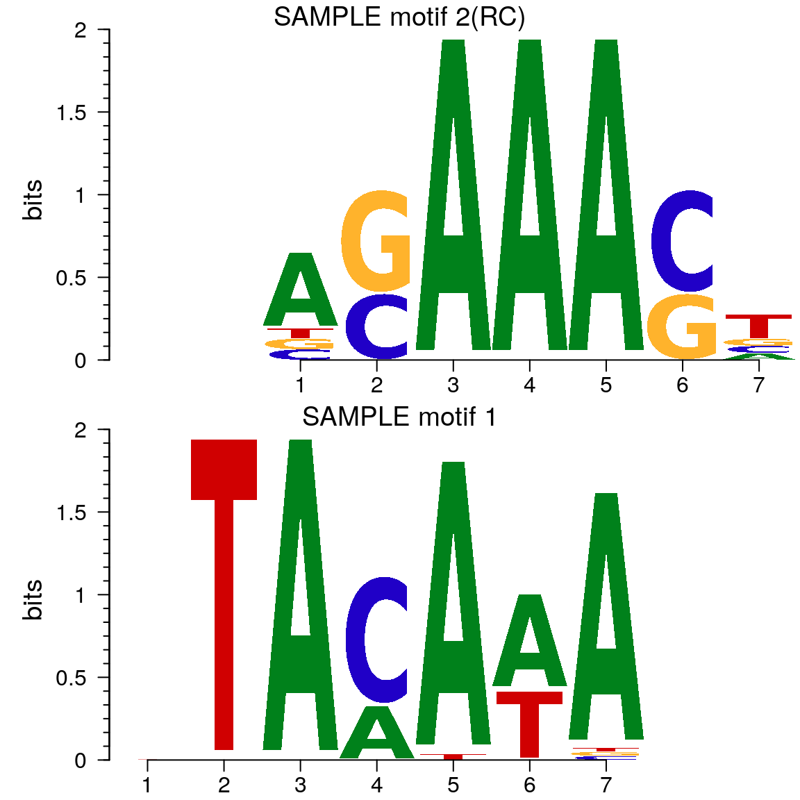
Motif of simulation data
Find peaks with bi-directional promoters
Bidirectional promoters are the DNA regions located between TSS of two adjacent genes that are transcribed on opposite directions and often co-regulated by this shared promoter region. Here is an example to find peaks near bi-directional promoters.
bdp <- peaksNearBDP(overlaps, annoDataTxDb, maxgap=5000)
c(bdp$percentPeaksWithBDP,
  bdp$n.peaks,
  bdp$n.peaksWithBDP)
## [1] 0.05421687 166.00000000 9.00000000head(bdp$peaksWithBDP, n=2)
## GRangesList object of length 2:
## $`4`
## GRanges object with 2 ranges and 10 metadata columns:
##      seqnames        ranges strand |                  peakNames     score
##         <Rle>     <IRanges>  <Rle> |            <CharacterList> <numeric>
##   X4     chr1 856361-856999      * | gr1__MACS_peak_17,gr2__005     54.69
##   X4     chr1 856361-856999      * | gr1__MACS_peak_17,gr2__005     54.69
##        bdp_idx        peak     feature feature.ranges feature.strand  distance
##      <integer> <character> <character>      <IRanges>          <Rle> <integer>
##   X4         4          X4   100130417  852953-854817              -      1543
##   X4         4          X4      148398  860530-879961              +      3530
##      insideFeature distanceToSite
##        <character>      <integer>
##   X4      upstream           1543
##   X4      upstream           3530
##   -------
##   seqinfo: 1 sequence from an unspecified genome; no seqlengths
##
## $`5`
## GRanges object with 2 ranges and 10 metadata columns:
##      seqnames        ranges strand |                  peakNames     score
##         <Rle>     <IRanges>  <Rle> |            <CharacterList> <numeric>
##   X5     chr1 859315-860144      * | gr2__006,gr1__MACS_peak_18    81.485
##   X5     chr1 859315-860144      * | gr2__006,gr1__MACS_peak_18    81.485
##        bdp_idx        peak     feature feature.ranges feature.strand  distance
##      <integer> <character> <character>      <IRanges>          <Rle> <integer>
##   X5         5          X5   100130417  852953-854817              -      4497
##   X5         5          X5      148398  860530-879961              +       385
##      insideFeature distanceToSite
##        <character>      <integer>
##   X5      upstream           4497
##   X5      upstream            385
##   -------
##   seqinfo: 1 sequence from an unspecified genome; no seqlengths
Determine if there is a significant overlap among multiple sets of peaks
Given two or more peak lists from different TFs, one may be interested in finding whether DNA binding profile of those TFs are correlated, and if correlated, what is the common binding pattern.
Here we will show how to compare binding profiles from multiple transcription factors (TFs) by ChIP-seq sample data of TAF, YY1 and Tead4 from mouse.
path <- system.file("extdata", package="ChIPpeakAnno")
files <- dir(path, "broadPeak")
data <- sapply(file.path(path, files), toGRanges, format="broadPeak")
(names(data) <- gsub(".broadPeak", "", files))
## [1] "TAF" "Tead4" "YY1"Hypergeometric test
When we test the association between two sets of data based on hypergeometric distribution, the number of all potential binding sites is required. The parameter totalTest in the makeVennDiagram function indicates how many potential peaks in total will be used in the hypergeometric test. It should be larger than the largest number of peaks in the peak list. The smaller it is set, the more stringent the test is. The time used to calculate p-value does not depend on the value of the totalTest. For practical guidance on how to choose totalTest, please refer to the post. The following example makes an assumption that there are 3% of coding region plus promoter region. Because the sample data is only a subset of chromosome 2, we estimate that the total binding sites is 1/24 of possible binding region in the genome.
ol <- findOverlapsOfPeaks(data, connectedPeaks="keepAll")
averagePeakWidth <- mean(width(unlist(GRangesList(ol$peaklist))))
tot <- ceiling(3.3e+9 * .03 / averagePeakWidth / 24)
makeVennDiagram(ol, totalTest=tot, connectedPeaks="keepAll",
                fill=c("#CC79A7", "#56B4E9", "#F0E442"), # circle fill color
                col=c("#D55E00", "#0072B2", "#E69F00"), #circle border color
                cat.col=c("#D55E00", "#0072B2", "#E69F00"))
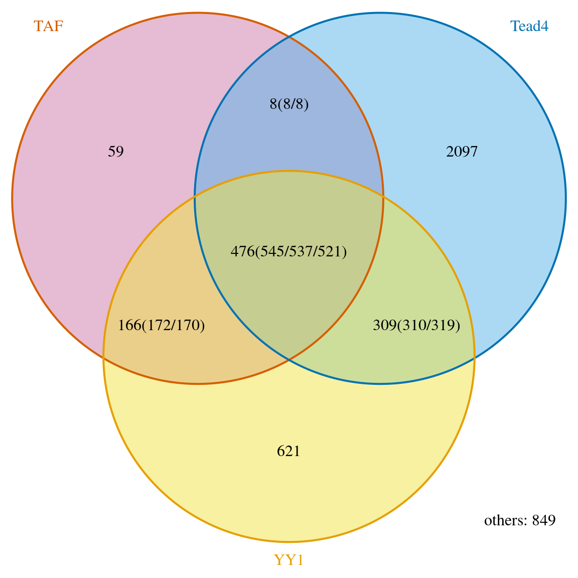
Venn diagram of overlaps.
## $p.value
##      TAF Tead4 YY1          pval
## [1,]   0     1   1  1.000000e+00
## [2,]   1     0   1 2.904297e-258
## [3,]   1     1   0  8.970986e-04
##
## $vennCounts
##      TAF Tead4 YY1 Counts count.TAF count.Tead4 count.YY1
## [1,]   0     0   0    849         0           0         0
## [2,]   0     0   1    621         0           0       621
## [3,]   0     1   0   2097         0        2097         0
## [4,]   0     1   1    309         0         310       319
## [5,]   1     0   0     59        59           0         0
## [6,]   1     0   1    166       172           0       170
## [7,]   1     1   0      8         8           8         0
## [8,]   1     1   1    476       545         537       521
## attr(,"class")
## [1] "VennCounts"
## see the difference if we set connectedPeaks to "keepFirstListConsistent" ## set connectedPeaks to keepFirstListConsistent will show consistent total ## number of peaks for the first peak list. makeVennDiagram(ol, totalTest=tot, connectedPeaks="keepFirstListConsistent", fill=c("#CC79A7", "#56B4E9", "#F0E442"), col=c("#D55E00", "#0072B2", "#E69F00"), cat.col=c("#D55E00", "#0072B2", "#E69F00"))
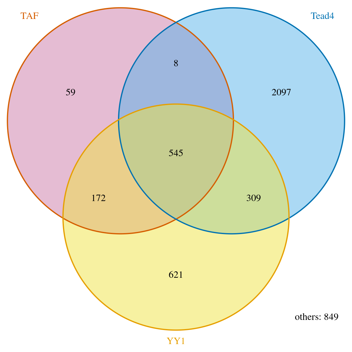
Venn diagram of overlaps for first TF.
## $p.value
##      TAF Tead4 YY1          pval
## [1,]   0     1   1  1.000000e+00
## [2,]   1     0   1 2.904297e-258
## [3,]   1     1   0  8.970986e-04
##
## $vennCounts
##      TAF Tead4 YY1 Counts count.TAF count.Tead4 count.YY1
## [1,]   0     0   0    849         0           0         0
## [2,]   0     0   1    621         0           0       621
## [3,]   0     1   0   2097         0        2097         0
## [4,]   0     1   1    309         0         310       319
## [5,]   1     0   0     59        59           0         0
## [6,]   1     0   1    166       172           0       170
## [7,]   1     1   0      8         8           8         0
## [8,]   1     1   1    476       545         537       521
## attr(,"class")
## [1] "VennCounts"
Permutation test
The above hypergeometric test requires users to input an estimate of the total potential binding sites for a given TF. To circumvent this requirement, we implemented a permutation test called peakPermTest. Before performing a permutation test, users need to generate random peaks using the distribution discovered from the input peaks for a given feature type (transcripts or exons), to make sure the binding positions relative to features, such as TSS and geneEnd, and the width of the random peaks follow the distribution of that of the input peaks.
Alternatively, a peak pool representing all potential binding sites can be created with associated binding probabilities for random peak sampling using the preparePool function. Here is an example to build a peak pool for human genome using the transcription factor binding site clusters (V3) (see ?wgEncodeTfbsV3) downloaded from ENCODE with the HOT spots (?HOT.spots) removed. HOT spots are the genomic regions with high probability of being bound by many TFs in ChIP-seq experiments. We suggest remove those HOT spots from the peak lists before performing permutation test to avoid the overestimation of the association between the two input peak lists. Users can also choose to remove ENCODE blacklist for a given species. The blacklists were constructed by identifying consistently problematic regions over independent cell lines and types of experiments for each species in the ENCODE and modENCODE datasets. Please note that some of the blacklists may need to be converted to the correct genome assembly using liftover utility.
Following are the sample codes to do the permutation test using the permTest function:
    data(HOT.spots)
    data(wgEncodeTfbsV3)
    hotGR <- reduce(unlist(HOT.spots))
    removeOl <- function(.ele){
        ol <- findOverlaps(.ele, hotGR)
        if(length(ol)>0) .ele <- .ele[-unique(queryHits(ol))]
        .ele
    }
    TAF <- removeOl(data[["TAF"]])
    TEAD4 <- removeOl(data[["Tead4"]])
    YY1 <- removeOl(data[["YY1"]])
    # we subset the pool to save demo time
    set.seed(1)
    wgEncodeTfbsV3.subset <-
        wgEncodeTfbsV3[sample.int(length(wgEncodeTfbsV3), 2000)]
    pool <- new("permPool", grs=GRangesList(wgEncodeTfbsV3.subset), N=length(YY1))
    pt1 <- peakPermTest(YY1, TEAD4, pool=pool, seed=1, force.parallel=FALSE)
    plot(pt1)
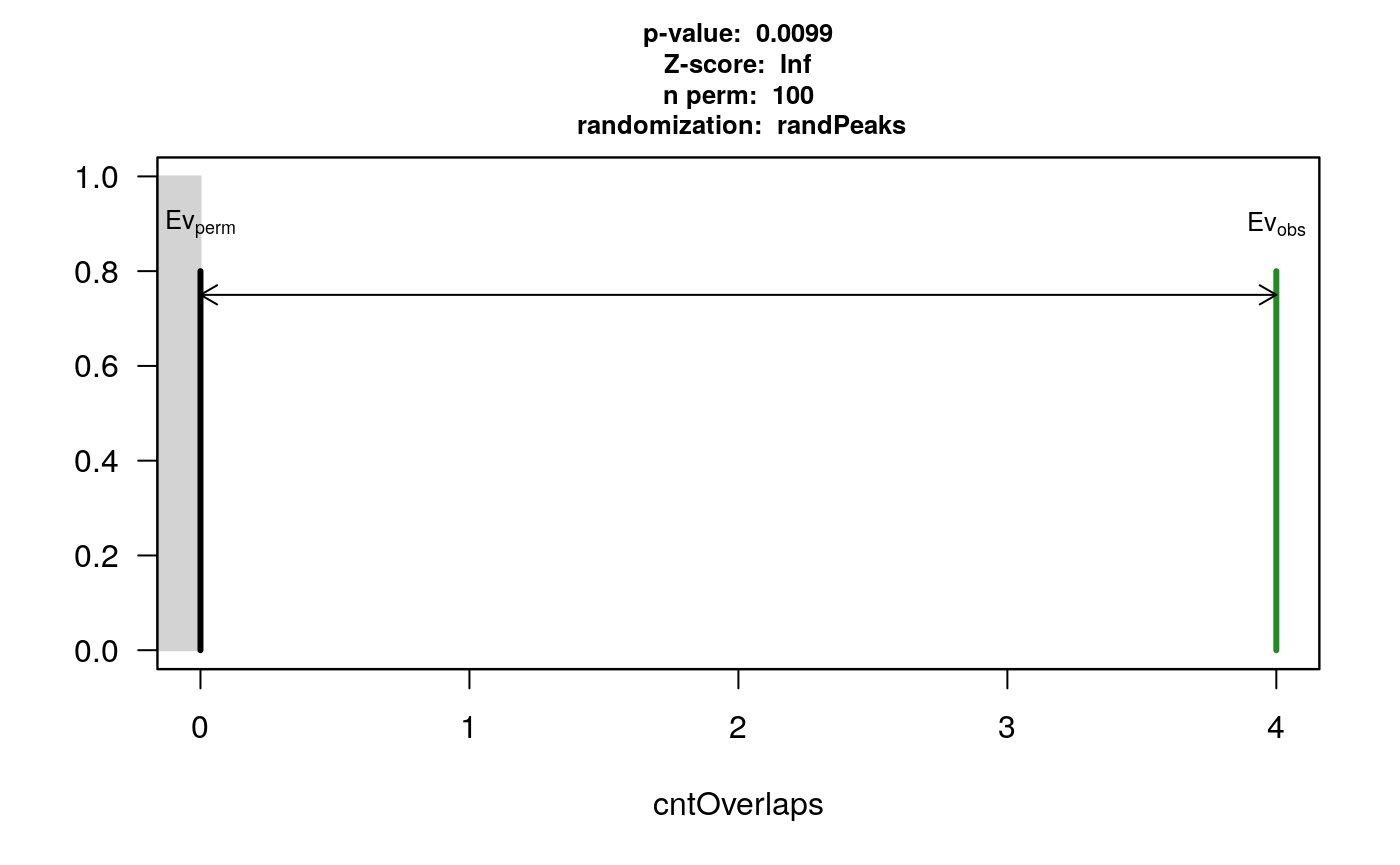
permutation test for YY1 and TEAD4
    pt2 <- peakPermTest(YY1, TAF, pool=pool, seed=1, force.parallel=FALSE)
    plot(pt2)
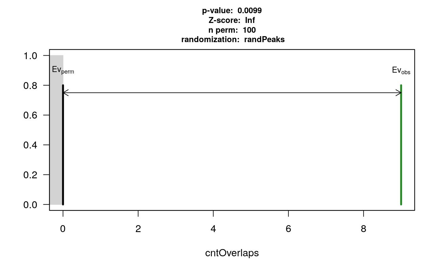
permutation test for YY1 and TAF
Metagene analysis for given feature/peak ranges
You can easily visualize and compare the binding patterns of raw signals of multiple ChIP-Seq experiments using function featureAlignedHeatmap and featureAlignedDistribution.
features <- ol$peaklist[[length(ol$peaklist)]]
feature.recentered <- reCenterPeaks(features, width=4000)
## here we also suggest importData function in bioconductor trackViewer package
## to import the coverage.
## compare rtracklayer, it will save you time when handle huge dataset.
library(rtracklayer)
files <- dir(path, "bigWig")
if(.Platform$OS.type != "windows"){
    cvglists <- sapply(file.path(path, files), import,
                       format="BigWig",
                       which=feature.recentered,
                       as="RleList")
}else{## rtracklayer can not import bigWig files on Windows
    load(file.path(path, "cvglist.rds"))
}
names(cvglists) <- gsub(".bigWig", "", files)
feature.center <- reCenterPeaks(features, width=1)
sig <- featureAlignedSignal(cvglists, feature.center,
                            upstream=2000, downstream=2000)
##Because the bw file is only a subset of the original file,
##the signals are not exists for every peak.
keep <- rowSums(sig[[2]]) > 0
sig <- sapply(sig, function(.ele) .ele[keep, ], simplify = FALSE)
feature.center <- feature.center[keep]
heatmap <- featureAlignedHeatmap(sig, feature.center,
                                 upstream=2000, downstream=2000,
                                 upper.extreme=c(3,.5,4))
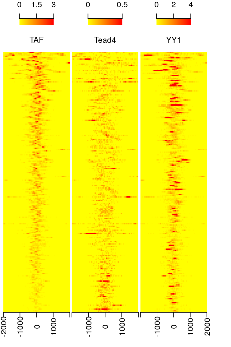
Heatmap of aligned features sorted by signal of TAF
featureAlignedDistribution(sig, feature.center,
                           upstream=2000, downstream=2000,
                           type="l")
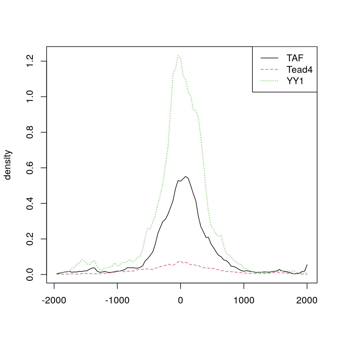
Distribution of aligned features