Introduction
A sequence motif is a short sequence conserved in multiple amino acid or nucleic acid sequences with biological significance such as DNA binding sites, where transcription factors (TFs) bind and catalytic sites in enzymes. Motifs are often represented as position count matrix (PCM)(Table @ref(tab:motifStackPCM)), position frequency matrix (PFM)(Table @ref(tab:motifStackPFM)) or position weight matrix (PWM) (reviewed in1–3). Sequence logos, based on information theory or probability theory, have been used as a graphical representation of sequence motifs to depict the frequencies of bases or amino acids at each conserved position4–8.
| A | 1 | 1 | 23 | 22 | 1 | 2 |
| C | 19 | 16 | 0 | 0 | 2 | 4 |
| G | 2 | 4 | 0 | 1 | 19 | 15 |
| T | 1 | 2 | 0 | 0 | 1 | 2 |
| A | 0.04 | 0.04 | 1 | 0.96 | 0.04 | 0.09 |
| C | 0.83 | 0.70 | 0 | 0.00 | 0.09 | 0.17 |
| G | 0.09 | 0.17 | 0 | 0.04 | 0.83 | 0.65 |
| T | 0.04 | 0.09 | 0 | 0.00 | 0.04 | 0.09 |
High-throughput experimental approaches have been developed to identify binding sequences for a large number of TFs in several organisms. The experimental methods include protein binding microarray (PBM)9, bacterial one-hybrid (B1H)10, systematic evolution of ligands by exponential enrichment (SELEX)11,12, High-Throughput (HT) SELEX13, and selective microfluidics-based ligand enrichment followed by sequencing (SMiLE-seq)14. Several algorithms have been developed to discover motifs from the binding sequences, identified by the above experimental methods. For example, MEME Suite15 has been widely used to construct motifs for B1H and SELEX data, while Seed-and-Wobble (SW)16, Dream517, and BEEML18 have been used to generate motifs for PBM data.
Visualization tools have been developed for representing a sequence motif as individual sequence logo, such as weblogo7and seqlogo19. To facilitate the comparison of multiple motifs, several motif alignment and clustering tools have been developed such as Tomtom20, MatAlign21, and STAMP22. However, these tools are lacking flexibility in dispalying the similarities or differences among motifs.
The motifStack package23 is designed for for the graphic representation of multiple motifs with their similarities or distances depicted. It provides the flexibility for users to customize the clustering and graphic parameters such as distance cutoff, the font family, colors, symbols, layout styles, and ways to highlight different regions or branches.
In this workshop, we will demonstrate the features and flexibility of motifStack for visualizing the alignment of multiple motifs in various styles. In addition, we will illustrate the utility of motifStack for providing insights into families of related motifs using several large collections of homeodomain (HD) DNA binding motifs from human, mouse and fly. Furthermore, we will show how motifStack facilitated the discovery that changing the computational method used to build motifs from the same binding data can lead to artificial segregation of motifs for identical TFs using the same motif alignment method.
Installation
BiocManager is used to install the released version of motifStack.
To install the development version of motifStack, please try
packageVersion("motifStack")
## [1] '1.33.8'Please note that starting from version 1.28.0, motifStack requires cario (>=1.6) instead of ghostscript which is for a lower version of motifStack. The capabilities function could be used to check capablilities of cario for current R session. If motifStack version number is smaller than 1.28.0, the full path to the executable ghostscript must be available for R session. Starting from version 1.33.2, motifStack does not require cario or ghostscript any more. It will use cario if cario (>=1.6) is installed or use ghostscript if gs command is available. Otherwise, motifStack will use embed font to plot the sequence logo.
In this tutorial, we will illustrate the functionalities of motifStack available in version >=1.33.3.
if(packageVersion("motifStack")<"1.33.3"){
  BiocManager::install("jianhong/motifStack", upgrade="never",
                       build_vignettes=TRUE, force = TRUE)
}
Inputs of motifStack
The inputs of motifStack are one or more motifs represented as PCM or PFM. Motifs in PFM format are available in most of the motif databases such as TRANSFAC24, JASPAR25, CIS-BP26 and HOCOMOCO27. More databases could be found at http://meme-suite.org/db/motifs.
In addition, MotifDb package contains a collection of DNA-binding sequence motifs in PFM format. 9933 PFMs were collected from 11 sources: cisbp_1.0226, FlyFactorSurvey28, HOCOMOCO27, HOMER29, hPDI30, JASPAR25, Jolma201331, ScerTF32, stamlab33, SwissRegulon34 and UniPROBE9.
## MotifDb object of length 12
## | Created from downloaded public sources: 2013-Aug-30
## | 12 position frequency matrices from 8 sources:
## |        HOCOMOCOv10:    2
## | HOCOMOCOv11-core-A:    2
## |        JASPAR_2014:    1
## |        JASPAR_CORE:    1
## |         jaspar2016:    1
## |         jaspar2018:    2
## |          jolma2013:    1
## |       SwissRegulon:    2
## | 1 organism/s
## |           Hsapiens:   12
## Hsapiens-HOCOMOCOv10-CTCFL_HUMAN.H10MO.A
## Hsapiens-HOCOMOCOv10-CTCF_HUMAN.H10MO.A
## Hsapiens-HOCOMOCOv11-core-A-CTCFL_HUMAN.H11MO.0.A
## Hsapiens-HOCOMOCOv11-core-A-CTCF_HUMAN.H11MO.0.A
## Hsapiens-JASPAR_CORE-CTCF-MA0139.1
## ...
## Hsapiens-jaspar2018-CTCF-MA0139.1
## Hsapiens-jaspar2018-CTCFL-MA1102.1
## Hsapiens-jolma2013-CTCF
## Hsapiens-SwissRegulon-CTCFL.SwissRegulon
## Hsapiens-SwissRegulon-CTCF.SwissRegulonpfm[["Hsapiens-jolma2013-CTCF"]]
##            1          2          3           4            5           6
## A 0.45533165 0.17369230 0.00000000 0.005067300 0.0623177134 0.004530681
## C 0.04584383 0.02478455 0.94098399 0.000000000 0.9324324324 0.995469319
## G 0.14550798 0.75930256 0.00000000 0.988123515 0.0007777562 0.000000000
## T 0.35331654 0.04222059 0.05901601 0.006809184 0.0044720980 0.000000000
##            7           8            9          10         11          12
## A 0.50758368 0.007861919 0.0000000000 0.002594670 0.76366002 0.007318263
## C 0.45336471 0.640791614 0.9998872985 0.003436185 0.02095981 0.131403480
## G 0.01804393 0.000000000 0.0001127015 0.001612903 0.11744724 0.799154334
## T 0.02100767 0.351346467 0.0000000000 0.992356241 0.09793293 0.062123923
##           13           14         15          16        17
## A 0.01376768 0.0002326934 0.03978832 0.151956584 0.3644148
## C 0.38797773 0.0000000000 0.01117209 0.281976578 0.3105268
## G 0.00000000 0.9856893543 0.73137985 0.008169095 0.2124384
## T 0.59825459 0.0140779523 0.21765974 0.557897744 0.1126200
The plotMotifLogo function can be used to plot sequence logo for motifs in PFM format (Figure @ref(fig:motifStackplotMotifLogo)). As default, the nucleotides in a sequence logo will be drawn proportional to their information content (IC)8.
library(motifStack)
plotMotifLogo(pfm[["Hsapiens-jolma2013-CTCF"]])
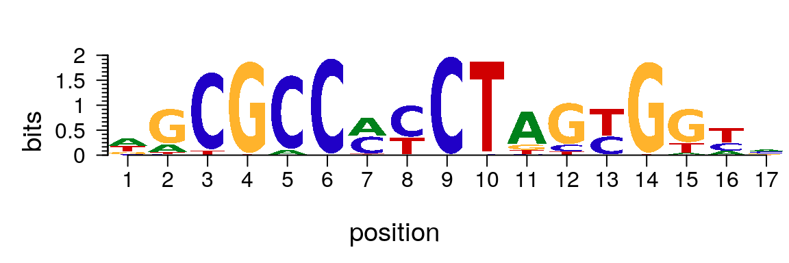
Plot sequence logo for motif in PFM format.
A PFM can be formated as an pfm object which is the preferred format for motifStack (Figure @ref(fig:motifStackplotMotifPFM)).
matrix.bin <- MotifDb::query(MotifDb, "bin_SANGER")
motif <- new("pfm", mat=matrix.bin[[1]], name=names(matrix.bin)[1])
motifStack(motif)
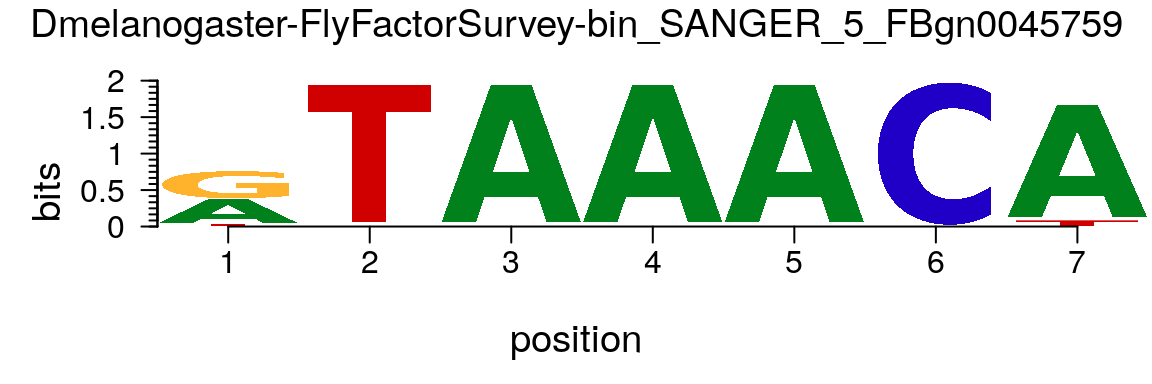
Plot sequence logo for a pfm object.
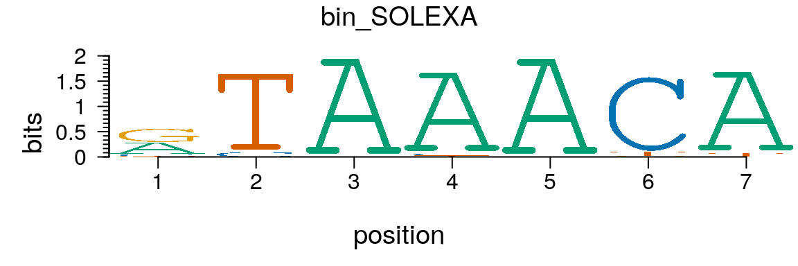
Similary, a PCM can be converted to a pcm object easily (Figure @ref(fig:motifStackplotMotifPCM)).
path <- system.file("extdata", package = "motifStack")
(pcm <- read.table(file.path(path, "bin_SOLEXA.pcm")))
##   V1 V2  V3   V4   V5   V6   V7  V8   V9
## 1  A  | 462    0 1068 1025 1068   0 1019
## 2  C  |  71   60    0   24    0 993    0
## 3  G  | 504    0    0    0    0  12    0
## 4  T  |  31 1008    0   19    0  63   49
pcm <- pcm[,3:ncol(pcm)] rownames(pcm) <- c("A","C","G","T") # must have rownames motif <- new("pcm", mat=as.matrix(pcm), name="bin_SOLEXA") plot(motif)
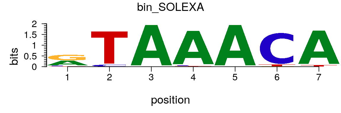
Plot sequence logo for a pcm object.
In addition, importMatrix function can be used to import the motifs into a pcm or pfm object from files exported by TRANSFAC24, JASPAR25 or CIS-BP26.
motifs <- importMatrix(dir(path, "*.pcm", full.names = TRUE),
                       format = "pcm", to = "pcm")
motifStack(motifs)
Plot sequence logo for data imported by importMatrix
Plot single sequence logo
motifStack can be used to plot DNA/RNA sequence logo, affinity logo and amino acid sequence logo. It provides the flexibility for users to customize the graphic parameters such as the font family, symbol colors and markers. Different from most of the sequence logo plotting tools, motifStack does not need to pre-define the path for plotting. It depends on grImport/235 package to import fonts into a path, which provides the power of motifStack more flexibility.
Plot a DNA/RNA/amino acid sequence logo
To plot an RNA sequence logo, simply change the rowname of the matrix from “T” to “U” (Figure @ref(fig:motifStackplotRNAmotif)).
rna <- pcm
rownames(rna)[4] <- "U"
RNA_motif <- new("pcm", mat=as.matrix(rna), name="RNA_motif")
plot(RNA_motif)
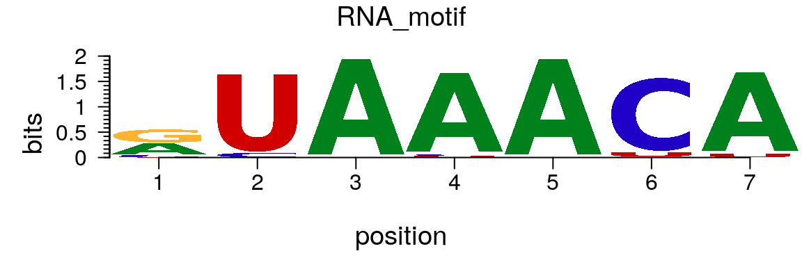
Plot an RNA sequence logo.
If the PFM of amino acid sequence motif is provided, motifStack can be used to draw amino acid sequence logo (Figure @ref(fig:motifStackplotAAmotif)).
library(Biostrings)
protein<-read.table(system.file("extdata", "motifStack", "irg.txt",
                                package = "workshop2020"))
protein<-t(protein[,2:21])
rownames(protein) <- sort(AA_STANDARD)
protein_motif<-new("pcm", mat=protein, name="IRG",
                   color=colorset(alphabet="AA",colorScheme="chemistry"),
                   alphabet = "AA",
                   markers=list(new("marker", type="rect",
                                    start=c(1,27), stop=c(13,49),
                                    gp=gpar(col="#009E73", fill=NA, lty=2))))
plot(protein_motif)
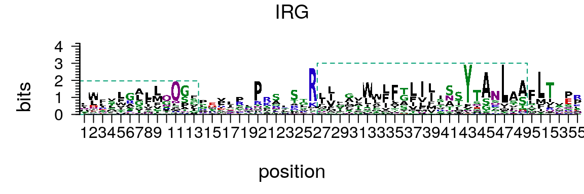
Plot amino acid sequence logo.
motifStack can also be used to plot other types of logos (Figure @ref(fig:motifStackplotANYlogo)).
m <- matrix(0, nrow = 10, ncol = 10,
            dimnames = list(strsplit("motifStack", "")[[1]],
                            strsplit("motifStack", "")[[1]]))
for(i in seq.int(10)) m[i, i] <- 1
ms <- new("pfm", mat=m, name="motifStack")
plot(ms)
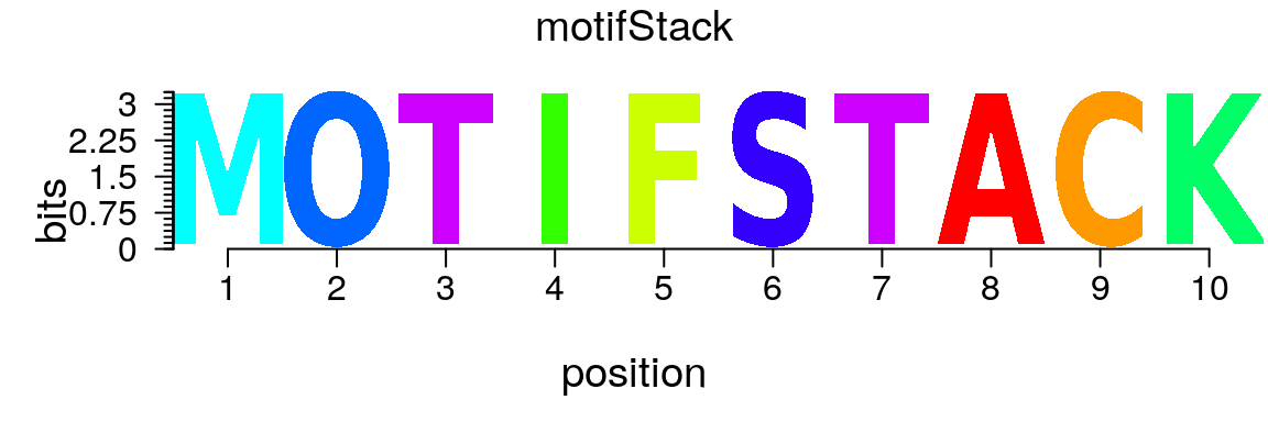
Plot a user-defined logo.
The sequence logo can be visulized with different fonts and colors (Figure @ref(fig:motifStackchangeFont)).
motif$color <- colorset(colorScheme = 'blindnessSafe')
plot(motif, font="mono,Courier", fontface="plain")
Plot sequence logo with different fonts and colors.
Plot sequence logo with specified regions highlighted using the markers slot
The markers slot of a pfm or pcm object can be assigned by a list of marker objects. There are three type of markers, “rect”, “line” and “text”. If markers slot is assigned, markers can be plotted (Figure @ref(fig:motifStackwithMarkers)).
markerRect <- new("marker", type="rect", start=6, stop=7,
                  gp=gpar(lty=2, fill=NA, col="orange", lwd=3))
markerRect2 <- new("marker", type="rect", start=2,
                   gp=gpar(lty=3, fill=NA, col="green", lwd=2))
markerLine <- new("marker", type="line", start=2, stop=7,
                  gp=gpar(lwd=2, col="darkblue"))
markerText <- new("marker", type="text", start=c(1, 5),
                  label=c("*", "core"), gp=gpar(cex=2, col="red"))
motif <- new("pcm", mat=as.matrix(pcm), name="bin_SOLEXA",
             markers=c(markerRect, markerLine, markerText, markerRect2))
plot(motif)
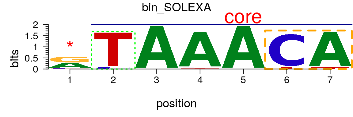
Plot a sequence logo with selected regions highlighted.
Plot motifs with ggplot2
Sequence logo can also be plotted by geom_motif function which is compatible with ggplot236 (Figure @ref(fig:motifStackggplot2)).
len <- length(motifs)
motifs[[1]]$markers <- list(markerRect2, markerRect)
df <- data.frame(x=.5, y=(seq.int(len)-.5)/len,
                 width=.75, height=1/(len+1))
df$motif <- motifs
library(ggplot2)
ggplot(df, aes(x=x, y=y, width=width, height=height, motif=motif)) +
  geom_motif(use.xy = TRUE) + theme_bw() + xlim(0, 1) + ylim(0, 1)
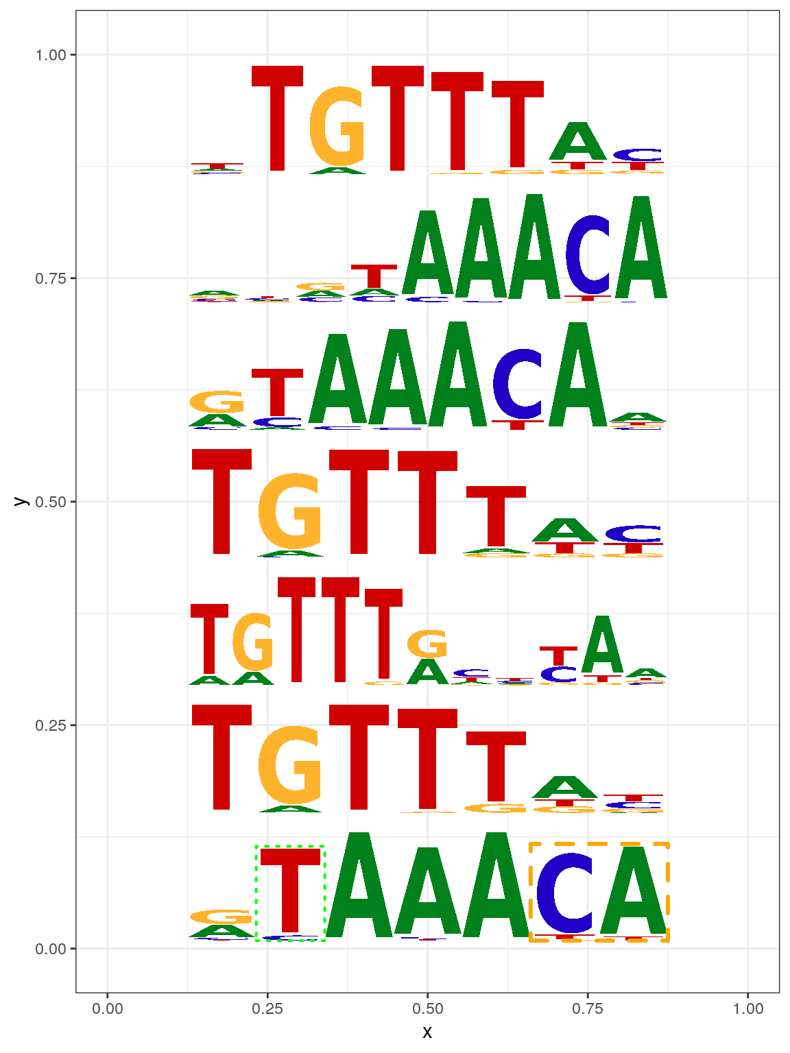
Plot sequence logo with ggplot2.
Plot multiple sequence logos
motifStack is designed to visulize the alignment of multiple motifs and facilitate the analysis of binding site diversity/conservation within families of TFs and evolution of binding sites among different species. There are many functions in motifStack such as plotMotifLogoStack, motifCloud, plotMotifStackWithRadialPhylog, motifPiles, and motifCircos for plotting motifs in different layouts, motifSignature for generating motif signatures by merging similar motifs. To make it easy to use, we created one workflow function called motifStack, which can be used to draw a single DNA, RNA or amino acid motif as a sequence logo, as well as to align motifs, generate motif signatures and plot aligned motifs as a stack, phylogeny tree, radial tree or cloud of sequence logos.
To align motifs, DNAmotifAlignment function implements Ungapped Smith–Waterman (local) alignment based on column comparison scores calculated by Kullback-Leibler distance37. DNAmotifAlignment requires the inputs be sorted by the distance of motifs. To get the sorted motifs for alignment, distances can be calculated using motifDistance in motIV (R implementation of STAMP22). Distances generated from MatAlign21 are also supported with a helper function ade4::newick2phylog38.
Plot sequence logo stack
As shown in above, motifStack function can be used to plot motifs as a stack of sequence logos easily. By setting the layout to “tree” (Figure @ref(fig:motifStacktreeLayout)) or “phylog” (Figure @ref(fig:motifStackphylogLayout)), motifStack will plot the stack of sequence logos with a linear tree.
motifStack(motifs, layout = "tree")
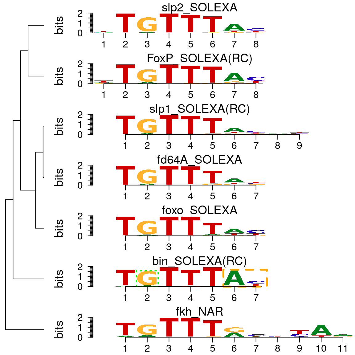
Plot sequence logo stack with tree layout.
motifStack(motifs, layout="phylog", f.phylog=.15, f.logo=0.25)
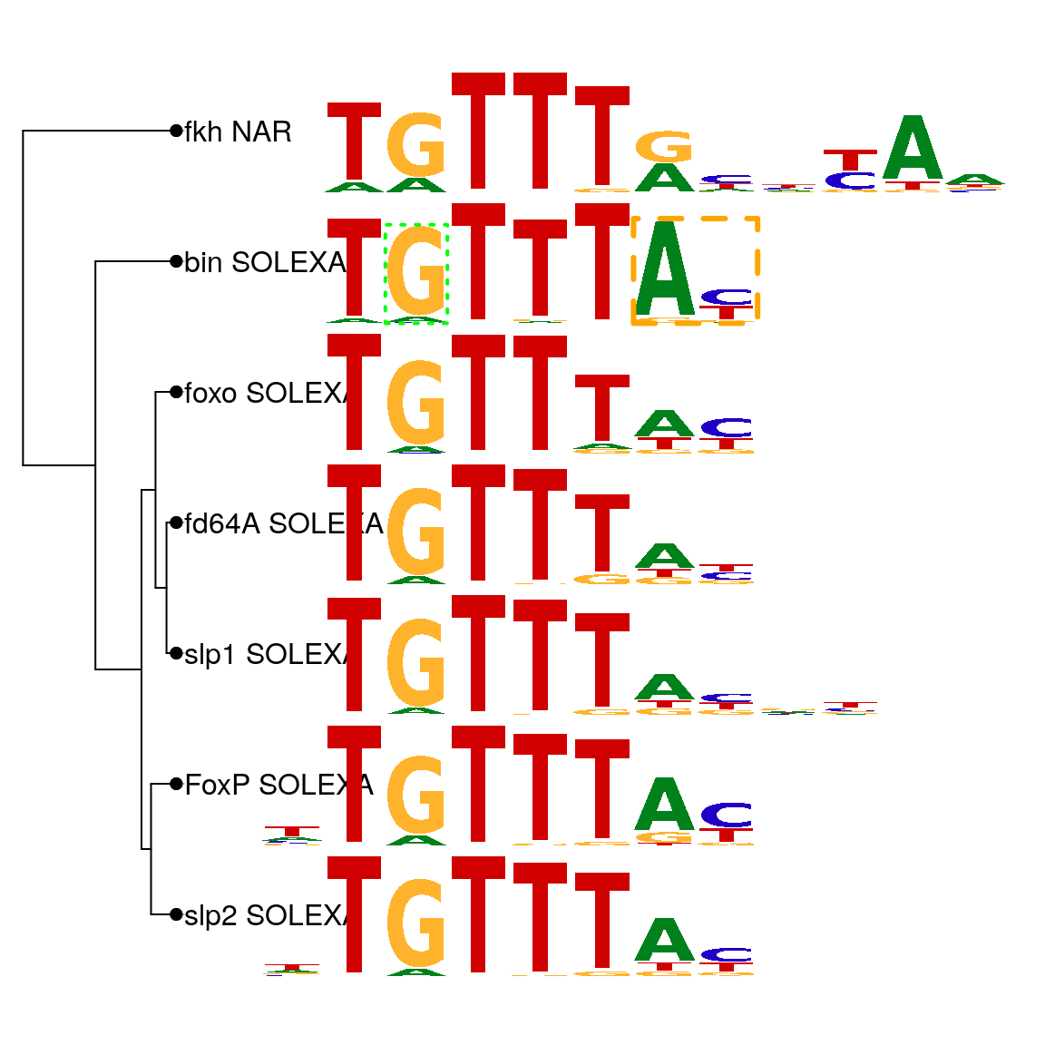
Plot sequence logo stack with phylog layout.
Even though the layout of “phylog” allows more motifs to be plotted comparing to the layout of “tree”, both layouts only allow small sets of motifs to be readily compared. However, moderate throughput analysis of TFs has generated 100s to 1000s of motifs, which make the visualization of their relationships more challenging. To reduce the total number of motifs depicted, clusters of highly similar motifs can be merged with the motifSignature function using a distance threshold. The distance threshold is user-determined; a low threshold will merge only extremely similar motifs while a higher threshold can group motifs with lower similarity.
library(MotifDb)
matrix.fly <- MotifDb::query(MotifDb, "FlyFactorSurvey")
motifs2 <- as.list(matrix.fly)
## format the name
names(motifs2) <- gsub("(_[\\.0-9]+)*_FBgn\\d+$", "",
                       elementMetadata(matrix.fly)$providerName)
names(motifs2) <- gsub("[^a-zA-Z0-9]", "_", names(motifs2))

motifs2 <- motifs2[unique(names(motifs2))]
## subsample motifs
set.seed(1)
pfms <- sample(motifs2, 50)
## cluster the motifs
hc <- clusterMotifs(pfms)
## convert the hclust to phylog object
library(ade4)
phylog <- hclust2phylog(hc)
## reorder the pfms by the order of hclust
leaves <- names(phylog$leaves)
pfms <- pfms[leaves]
## create a list of pfm objects
pfms <- mapply(pfms, names(pfms),
               FUN=function(.pfm, .name){
                 new("pfm",mat=.pfm, name=.name)})
## extract the motif signatures
motifSig <- motifSignature(pfms, phylog, cutoffPval = 0.0001, min.freq=1)
Logos for these merged motifs can be plotted on the same dendrograms, using the relative size of the logos to reflect the number of TFs that contribute to the merged motif. Compared with the original dendrogram, the number of TFs with similar motifs and the relationships between the merged motifs can be more easily compared. The 50 motifs shown in the original image are now shown as only 28 motif clusters/signatures, with the members of each cluster clearly indicated. By setting the colors of dendrogram via parameter col.tree, the colors of lable of leaves via parameter col.leaves, and the colors of annotation bar via parameter col.anno, motifPiles function can mark each motif with multiple annotation colors (Figure @ref(fig:motifStackmotifPiles)).
## get the signatures from object of motifSignature
sig <- signatures(motifSig)
## get the group color for each signature
gpCol <- sigColor(motifSig)

library(RColorBrewer)
color <- brewer.pal(12, "Set3")
## plot the logo stack with pile style.
motifPiles(phylog=phylog, pfms=pfms, pfms2=sig,
            col.tree=rep(color, each=5),
            col.leaves=rep(rev(color), each=5),
            col.pfms2=gpCol,
            r.anno=c(0.02, 0.03, 0.04),
            col.anno=list(sample(colors(), 50),
                          sample(colors(), 50),
                          sample(colors(), 50)),
            motifScale="logarithmic",
            plotIndex=TRUE)
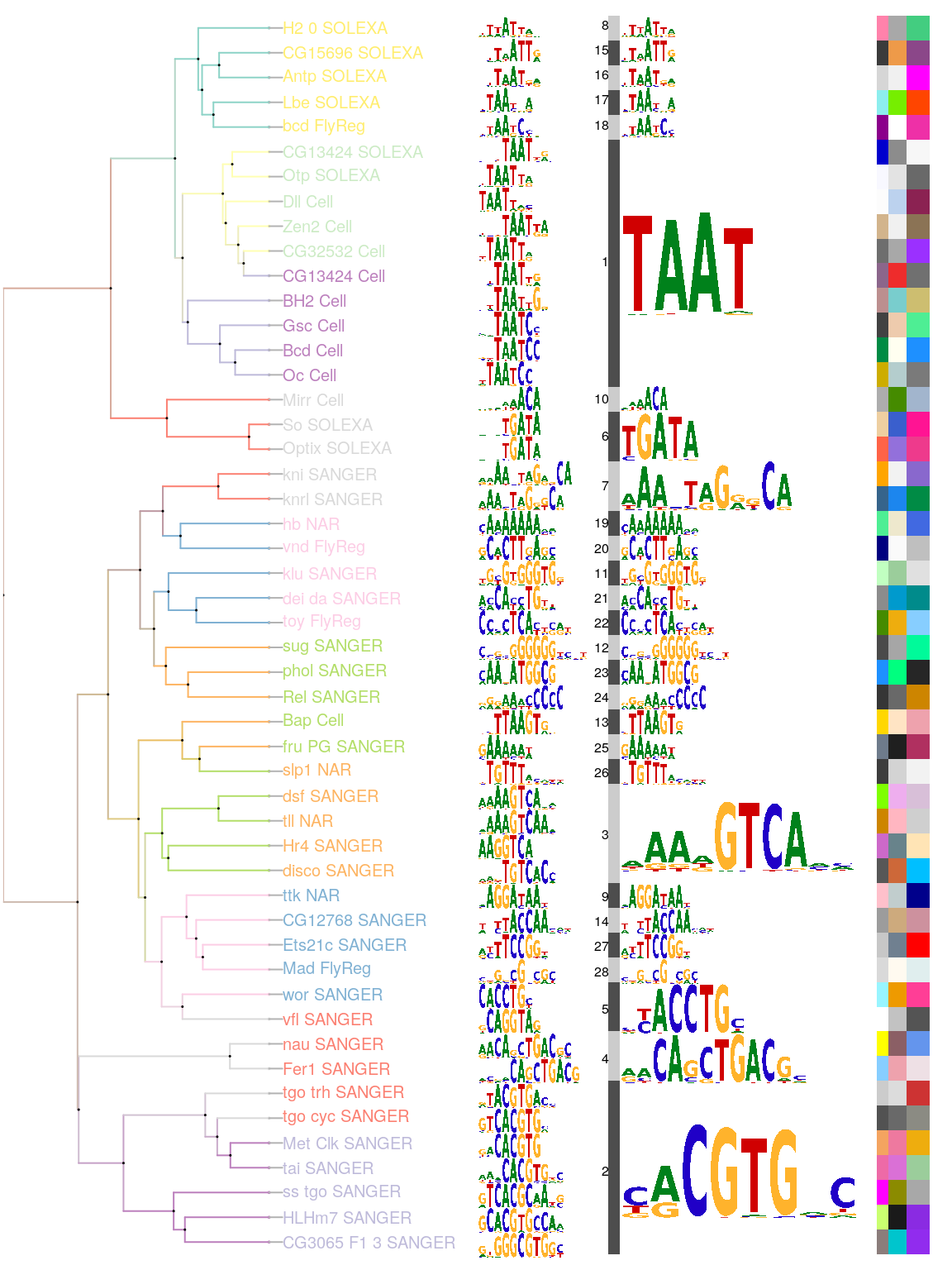
Plot sequence logo stack by motifPiles.
Plot sequence logo cloud
To emphasize the weight of motif signatures, motif signatures can be plotted as a circular (Figure @ref(fig:motifStackmotifCloud)) or rectanglular word clouds with motif size representing the number of motifs that contributed to the signature. The larger the motif size, the larger the number of motifs within that motif signature.
## draw the motifs with a word-cloud style.
motifCloud(motifSig, scale=c(6, .5), layout="cloud")
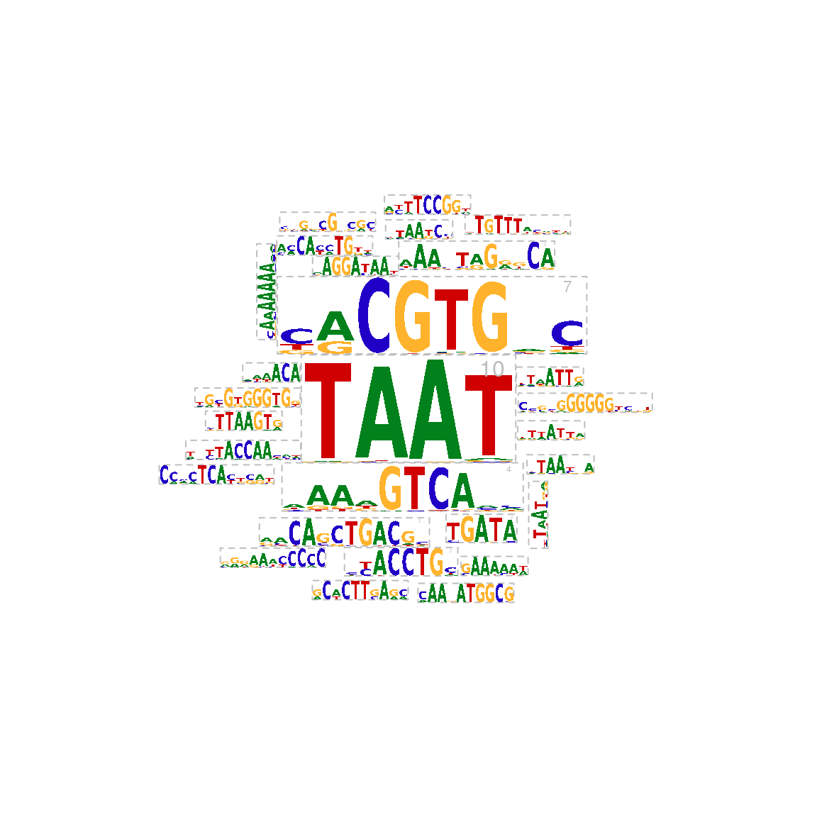
Plot sequence logo cloud.
Plot sequence logo circos
The sequence logo cloud will loose the cluster information. Plotting motifs as sequence logo circos is a good solution to visualize motif signatures with dendrogram (Figure @ref(fig:motifStackplotMotifStackWithRadialPhylog)).
## plot the logo stack with radial style.
plotMotifStackWithRadialPhylog(phylog=phylog, pfms=sig,
                              circle=0.4, cleaves = 0.3,
                              clabel.leaves = 0.5,
                              col.bg=rep(color, each=5), col.bg.alpha=0.3,
                              col.leaves=rep(rev(color), each=5),
                              col.inner.label.circle=gpCol,
                              inner.label.circle.width=0.03,
                              angle=350, circle.motif=1.2,
                              motifScale="logarithmic")
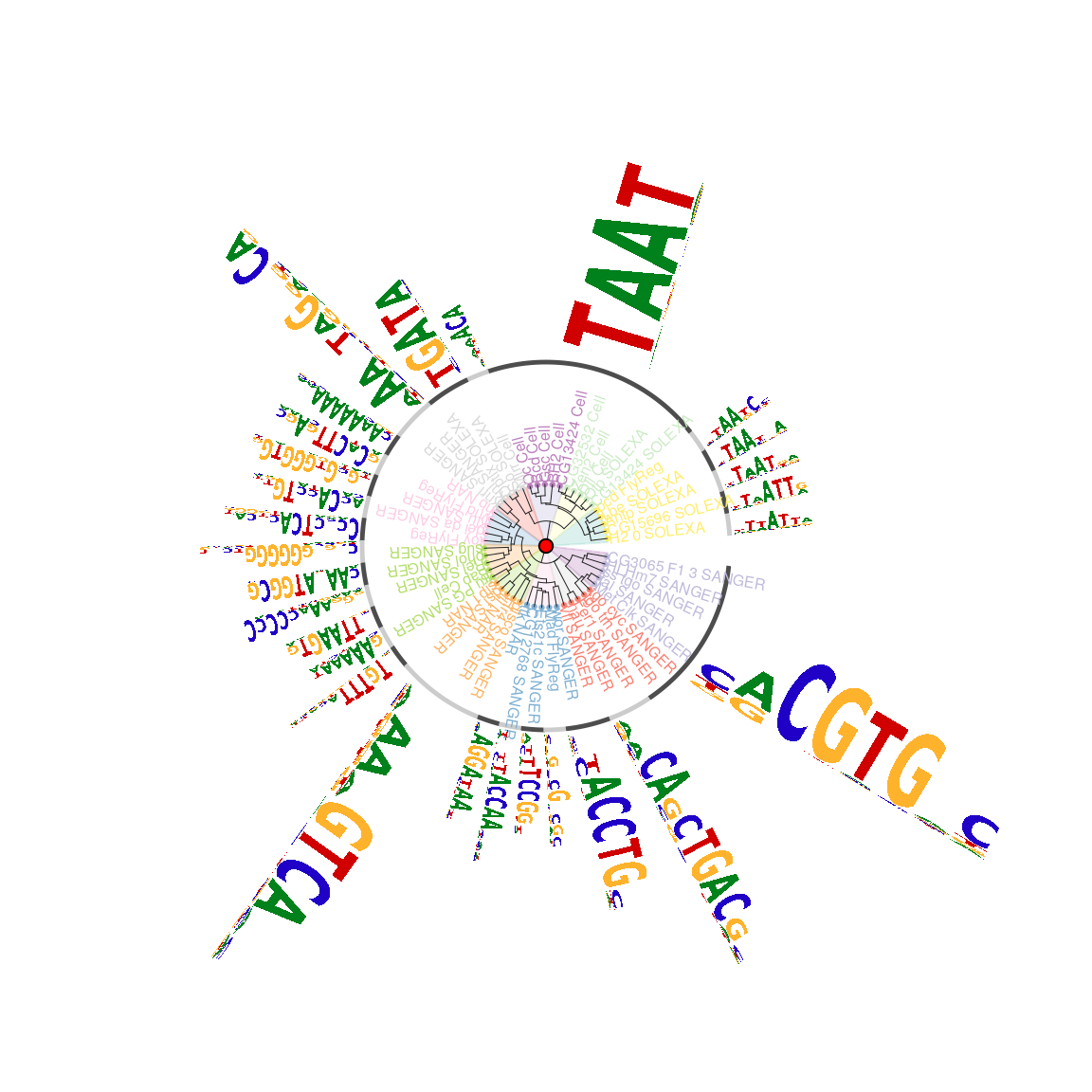
Plot sequence logo circos.
motifCircos function provide the possibility to plot the motif signatures with their original sequence logos in the circos style (Figure @ref(fig:motifStackmotifCircos)).
## plot the logo stack with cirsoc style.
motifCircos(phylog=phylog, pfms=pfms, pfms2=sig,
            col.tree.bg=rep(color, each=5), col.tree.bg.alpha=0.3,
            col.leaves=rep(rev(color), each=5),
            col.inner.label.circle=gpCol,
            inner.label.circle.width=0.03,
            col.outer.label.circle=gpCol,
            outer.label.circle.width=0.03,
            r.rings=c(0.02, 0.03, 0.04),
            col.rings=list(sample(colors(), 50),
                           sample(colors(), 50),
                           sample(colors(), 50)),
            angle=350, motifScale="logarithmic")
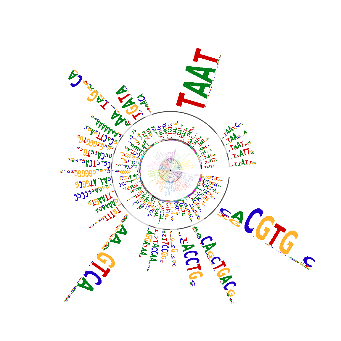
Plot sequence logo circos by motifCiros.
Plot motifs with d3.js in a webpage
Interactive plot can be generated using browseMotifs function which leverages the d3.js library. All motifs on the plot are draggable and the plot can be easily exported as a Scalable Vector Graphics (SVG) file.
browseMotifs(pfms = pfms, phylog = phylog, layout="radialPhylog",
             yaxis = FALSE, xaxis = FALSE, baseWidth=6, baseHeight = 15)
Plot motifs interactively.
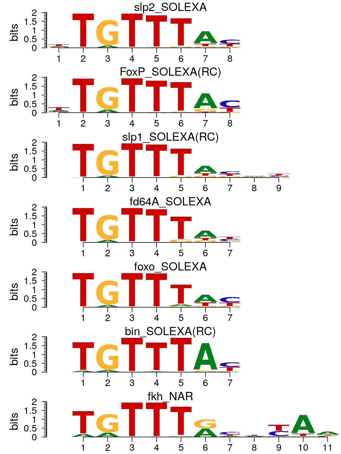
Plot fly data from different experimental methods
Following scripts will show how motifStack facilitated the discovery that changing the experiemntal method used to build motifs from the same binding data can lead to artificial segregation of motifs for identical TFs within a motif alignment. MatAlign21 was implemented in motifStack by following the code from http://stormo.wustl.edu/MatAlign/ to get the phylogenetic tree for given motifs. Compare to STAMP, MatAlign alignment method is superior for discriminating between the closely related motifs23.
Here we clustered motifs for a smaller set of fly HDs that were determined using four different experimental methods to measure DNA binding specificity, B1H, HT-SELEX, SMiLE-seq and PBM, to confirm that the motif generation method can impact clustering. As it shown in Figre @ref(fig:motifStackFlydata) B1H motifs from different lab tend to cluster with each other (motifs 17-26, 29,30, 36-45, 50-53, 60-68, 72-100, 102-143, 159-169, 172-180, 184, 185, 187, 188, 196, 197, 202-210, 238, 239) compared to PBM data (motifs ‘eve’ in blue). PMB data (motif 227-230, 240-247) tend to have lower IC, which may be introduced by computation methods23. HT-SELEX tend to have dimer (motif labels in red).
pfmpath <- system.file('extdata', "motifStack", "pfms", package = 'workshop2020')
pfmfiles <- dir(pfmpath, full.names = TRUE)
pfms <- lapply(pfmfiles, importMatrix, format="pfm", to="pfm")
pfms <- unlist(pfms)
## fix the name issue
names(pfms) <- gsub("\\.", "_", names(pfms))
pfms <- sapply(pfms, function(.ele){
  .ele@name <-gsub("\\.", "_", .ele@name)
  .ele
})
## get phylog
hc <- clusterMotifs(pfms)
library(ade4)
phylog <- ade4::hclust2phylog(hc)
leaves <- names(phylog$leaves)
motifs <- pfms[leaves]
motifSig <- motifSignature(motifs, phylog,
                           cutoffPval = 0.0001, min.freq=1)
sig <- signatures(motifSig)
gpCol <- sigColor(motifSig)

##set methods color
colorSet <- c("B1H_Mathelier"="#40E0D0", "B1H_Zhu"="#008080",
              "PBM_Busser"="brown", "PBM_Weirauch"="#F69156",
              "SELEX_Nitta"="blue",
              "SMiLE_seq_Isakova"="#D900D9")
methods <- factor(sub("^.*?__", "", leaves))
lev <- levels(methods)
levels(methods) <- colorSet[lev]
methods <- as.character(methods)

leaveNames <- gsub("__.*$", "", leaves)
leaveCol <- ifelse(leaveNames %in% c("unc_4", "hbn", "bsh", "Optix",
                                     "al", "PHDP", "CG32532", "CG11294"),
                   "#D55E00",
                   ifelse(leaveNames == "eve", "#0072B2", "#000000"))

## calculate average of top 8 position information content for each motif
icgp <- sapply(sapply(motifs, getIC), function(.ele)
  mean(sort(.ele, decreasing=TRUE)[1:min(8, length(.ele))]))
icgp.ranges <- range(icgp)
icgp <- cut(icgp, 10, labels=colorRampPalette(c("#009E73", "#000000", "#D55E00"))(10))
icgp.image <- as.raster(matrix(rev(levels(icgp)), ncol=1))
icgp <- as.character(icgp)

motifCircos(phylog=phylog, pfms=DNAmotifAlignment(motifs),
            col.tree.bg=methods, col.tree.bg.alpha=.3,
            r.rings=c(.05, .1), col.rings=list(icgp, rep("white", length(icgp))),
            col.inner.label.circle=gpCol, inner.label.circle.width=0.03,
            labels.leaves=leaveNames, col.leaves=leaveCol,
            cleaves=.1, r.tree=1.3, r.leaves=.2, clabel.leaves=.7,
            motifScale="logarithmic", angle=358,
            plotIndex=TRUE, IndexCex=.7)

legend(-2.4, 2.4, legend=names(colorSet),
       fill=highlightCol(colorSet, .3),
       border="white", lty=NULL, bty = "n")

text(2.05, 2.3, labels="Information Content")
rasterImage(icgp.image, 2, 1.8, 2.04, 2.2, interpolate = FALSE)
text(c(2.05, 2.05), c(1.8, 2.2), labels=format(icgp.ranges, digits=3), adj=0)
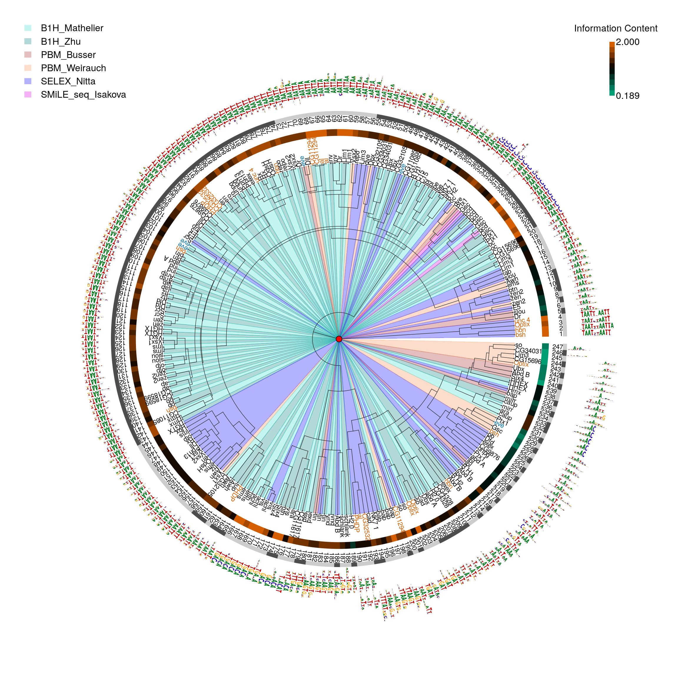
Fly data from different methods.
dagLogo: visualizing conserved amino acid sequence pattern in groups based on probability theory
As it shown in amino acid (AA) sequence logo (Figure @ref(fig:motifStackplotAAmotif)), the figure is somehow busy. To optimize the vigualization of amino acid logos, we developed the dagLogo package. This package can reduce the complex AA alphabets to group AAs of similar properties and provide statistical test for differential AA usage.
## load library dagLogo
library(dagLogo)
## prepare the proteome of fruitfly
proteome <- prepareProteomeByFTP(source = "UniProt",
                                 species = "Drosophila melanogaster")
## read the aligned sequences
library(Biostrings)
dat <- readAAStringSet(system.file("extdata", "motifStack", "irg.aligned.fa",
                                   package = "workshop2020"))
## prepare an object of dagPeptides Class from a Proteome object
## set the anchor to the most conserved position
seq <- formatSequence(seq = dat, proteome = proteome,
                      upstreamOffset = 25, downstreamOffset = 29)
## build the background model
bg_ztest <- buildBackgroundModel(seq, background = "wholeProteome",
                                 proteome = proteome, testType = "ztest")
## grouping based on the charge of AAs.
t <- testDAU(dagPeptides = seq, dagBackground = bg_ztest,
             groupingScheme = "chemistry_property_Mahler_group")
dagLogo(t, legend = TRUE)
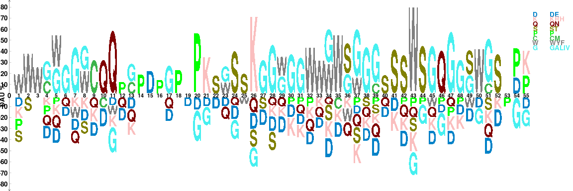
Visualizing conserved amino acid sequence pattern based on chemical properties
The package dagLogo allows users to use their own grouping scheme. To make the information more informatively for this special case, we assign the color of each group by their hydrophobicity.
## group of the aa by chemical properties
## order is them by hydrophobicity
group = list(
    RHK = c("K", "R", "H"),
    DE= c("D","E"),
    QN = c("Q", "N"),
    P = "P",
    WYF = c("W", "Y", "F"),
    ST  = c("S", "T"),
    CM = c("C", "M"),
    GALIV = c("G", "A", "L", "I", "V"))
## set the colors by color blindness safe gradient color
library(colorBlindness)
color <- Blue2Gray8Steps
names(color) <- names(group)
## assign symbols for each group
symbol <- substring(names(group), first = 1, last = 1)
names(symbol) <- names(group)
## Add a grouping scheme
## Please note that the user-supplied grouping is named
## as "custom_group" internally.
addScheme(color = color, symbol = symbol, group = group)
tt <- testDAU(dagPeptides = seq, dagBackground = bg_ztest,
              groupingScheme = "custom_group")
dagLogo(tt, legend = TRUE)
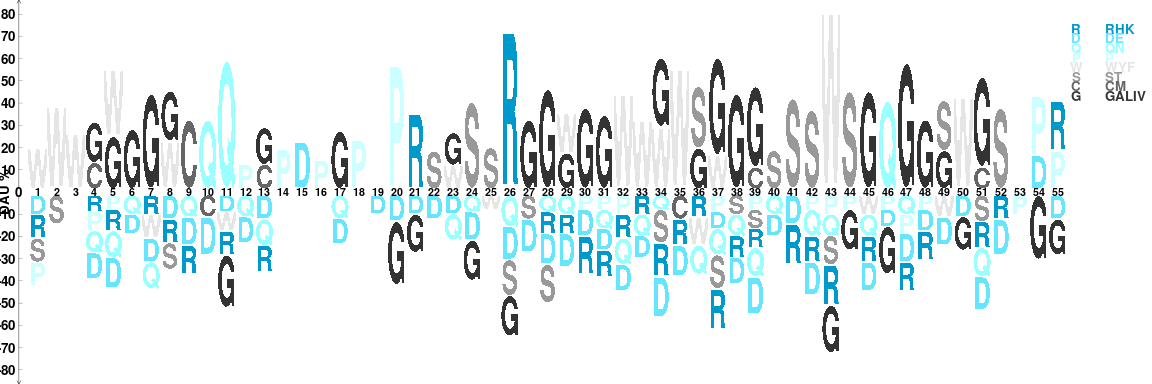
Visualizing conserved amino acid sequence pattern based on chemical properties and hydrophobicity
References
1. Das, M. K. & Dai, H.-K. A survey of dna motif finding algorithms. in BMC bioinformatics 8, S21 (BioMed Central, 2007).
2. Sandve, G. K., Abul, O., Walseng, V. & Drabløs, F. Improved benchmarks for computational motif discovery. BMC bioinformatics 8, 193 (2007).
3. Tompa, M. et al. Assessing computational tools for the discovery of transcription factor binding sites. Nature biotechnology 23, 137 (2005).
4. Schneider, T. D. & Stephens, R. M. Sequence logos: A new way to display consensus sequences. Nucleic acids research 18, 6097–6100 (1990).
5. Schneider, T. D. in Methods in enzymology 274, 445–455 (Elsevier, 1996).
6. Schneider, T. D. Strong minor groove base conservation in sequence logos implies dna distortion or base flipping during replication and transcription initiation. Nucleic acids research 29, 4881–4891 (2001).
7. Crooks, G. E., Hon, G., Chandonia, J.-M. & Brenner, S. E. WebLogo: A sequence logo generator. Genome research 14, 1188–1190 (2004).
8. Workman, C. T. et al. EnoLOGOS: A versatile web tool for energy normalized sequence logos. Nucleic acids research 33, W389–W392 (2005).
9. Newburger, D. E. & Bulyk, M. L. UniPROBE: An online database of protein binding microarray data on protein–dna interactions. Nucleic acids research 37, D77–D82 (2008).
10. Meng, X., Brodsky, M. H. & Wolfe, S. A. A bacterial one-hybrid system for determining the dna-binding specificity of transcription factors. Nature biotechnology 23, 988 (2005).
11. Ellington, A. D. & Szostak, J. W. In vitro selection of rna molecules that bind specific ligands. nature 346, 818 (1990).
12. Tuerk, C. & Gold, L. Systematic evolution of ligands by exponential enrichment: RNA ligands to bacteriophage t4 dna polymerase. Science 249, 505–510 (1990).
13. Hoinka, J. et al. Large scale analysis of the mutational landscape in ht-selex improves aptamer discovery. Nucleic acids research 43, 5699–5707 (2015).
14. Isakova, A. et al. SMiLE-seq identifies binding motifs of single and dimeric transcription factors. Nature methods 14, 316 (2017).
15. Bailey, T. L. et al. MEME suite: Tools for motif discovery and searching. Nucleic acids research 37, W202–W208 (2009).
16. Badis, G. et al. Diversity and complexity in dna recognition by transcription factors. Science 324, 1720–1723 (2009).
17. Weirauch, M. T. et al. Evaluation of methods for modeling transcription factor sequence specificity. Nature biotechnology 31, 126 (2013).
18. Zhao, Y. & Stormo, G. D. Quantitative analysis demonstrates most transcription factors require only simple models of specificity. Nature biotechnology 29, 480 (2011).
19. Bembom, O. SeqLogo: Sequence logos for dna sequence alignments. R package version 1,
20. Gupta, S., Stamatoyannopoulos, J. A., Bailey, T. L. & Noble, W. S. Quantifying similarity between motifs. Genome biology 8, R24 (2007).
21. Zhao, G. et al. Conserved motifs and prediction of regulatory modules in caenorhabditis elegans. G3: Genes, Genomes, Genetics 2, 469–481 (2012).
22. Mahony, S. & Benos, P. V. STAMP: A web tool for exploring dna-binding motif similarities. Nucleic acids research 35, W253–W258 (2007).
23. Ou, J., Wolfe, S. A., Brodsky, M. H. & Zhu, L. J. MotifStack for the analysis of transcription factor binding site evolution. Nature methods 15, 8 (2018).
24. Wingender, E. et al. TRANSFAC: An integrated system for gene expression regulation. Nucleic acids research 28, 316–319 (2000).
25. Sandelin, A., Alkema, W., Engström, P., Wasserman, W. W. & Lenhard, B. JASPAR: An open-access database for eukaryotic transcription factor binding profiles. Nucleic acids research 32, D91–D94 (2004).
26. Weirauch, M. T. et al. Determination and inference of eukaryotic transcription factor sequence specificity. Cell 158, 1431–1443 (2014).
27. Kulakovskiy, I. V. et al. HOCOMOCO: Towards a complete collection of transcription factor binding models for human and mouse via large-scale chip-seq analysis. Nucleic acids research 46, D252–D259 (2017).
28. Zhu, L. J. et al. FlyFactorSurvey: A database of drosophila transcription factor binding specificities determined using the bacterial one-hybrid system. Nucleic acids research 39, D111–D117 (2010).
29. Heinz, S. et al. Simple combinations of lineage-determining transcription factors prime cis-regulatory elements required for macrophage and b cell identities. Molecular cell 38, 576–589 (2010).
30. Xie, Z., Hu, S., Blackshaw, S., Zhu, H. & Qian, J. HPDI: A database of experimental human protein–dna interactions. Bioinformatics 26, 287–289 (2009).
31. Jolma, A. et al. DNA-binding specificities of human transcription factors. Cell 152, 327–339 (2013).
32. Spivak, A. T. & Stormo, G. D. ScerTF: A comprehensive database of benchmarked position weight matrices for saccharomyces species. Nucleic acids research 40, D162–D168 (2011).
33. Neph, S. et al. Circuitry and dynamics of human transcription factor regulatory networks. Cell 150, 1274–1286 (2012).
34. Pachkov, M., Erb, I., Molina, N. & Van Nimwegen, E. SwissRegulon: A database of genome-wide annotations of regulatory sites. Nucleic acids research 35, D127–D131 (2006).
35. Murrell, P. & others. Importing vector graphics: The grImport package for r. Journal of Statistical Software 30, 1–37 (2009).
36. Wickham, H. Ggplot2: Elegant graphics for data analysis. (Springer, 2016).
37. Roepcke, S., Grossmann, S., Rahmann, S. & Vingron, M. T-reg comparator: An analysis tool for the comparison of position weight matrices. Nucleic acids research 33, W438–W441 (2005).
38. Dray, S., Dufour, A.-B. & others. The ade4 package: Implementing the duality diagram for ecologists. Journal of statistical software 22, 1–20 (2007).