Figure 5
The Figure 5 is the showcase for geomeTriD package to
present multiple genomic signals along with 3D models for topologically
associating domain (TADs).
Load Libraries
library(geomeTriD)
library(geomeTriD.documentation)
library(GenomicRanges)
library(TxDb.Hsapiens.UCSC.hg38.knownGene)
library(org.Hs.eg.db)
library(clusterCrit)
library(colorRamps)
Load data and annotations
The data were from diffraction-limited experiments for IMR90 cells.
## xyz is from diffraction-limited experiments but not the actual xyz cords of STORM experiments.
xyz <- read.csv('https://github.com/BogdanBintu/ChromatinImaging/raw/refs/heads/master/Data/IMR90_chr21-28-30Mb.csv', skip = 1)
## split the XYZ for each chromosome
xyz.s <- split(xyz[, -1], xyz$Chromosome.index)
head(xyz.s[[1]])
## Segment.index Z X Y
## 1 1 3090 135130 50097
## 2 2 3096 135094 50393
## 3 3 3216 135329 49882
## 4 4 3209 135166 50006
## 5 5 3153 135046 50028
## 6 6 3285 134862 49955
range <- GRanges("chr21:28000001-29200000")
### get feature annotations
feature.gr <- getFeatureGR(txdb = TxDb.Hsapiens.UCSC.hg38.knownGene,
                           org = org.Hs.eg.db,
                           range = range)
## 2169 genes were dropped because they have exons located on both strands of
## the same reference sequence or on more than one reference sequence, so cannot
## be represented by a single genomic range.
## Use 'single.strand.genes.only=FALSE' to get all the genes in a GRangesList
## object, or use suppressMessages() to suppress this message.## 'select()' returned 1:1 mapping between keys and columns
### get genomic signals, we will use called peaks
colorSets <- c(CTCF="cyan",YY1="yellow",
               RAD21="red", SMC1A="green", SMC3="blue")
prefix <- 'https://www.encodeproject.org/files/'
imr90_url <- c(ctcf = 'ENCFF203SRF/@@download/ENCFF203SRF.bed.gz',
               smc3 = 'ENCFF770ISZ/@@download/ENCFF770ISZ.bed.gz',
               rad21 = 'ENCFF195CYT/@@download/ENCFF195CYT.bed.gz')
imr90_urls <- paste0(prefix, imr90_url)
names(imr90_urls) <- names(imr90_url)
# download the files and import the signals
imr90_genomicSigs <- importSignalFromUrl(imr90_urls, range = range,
                                         cols = list(
                                           'ctcf'=c('#111100', 'cyan'),
                                           'smc3'=c('#000011', 'blue'),
                                           'rad21'=c('#110000', 'red')),
                                         format = 'BED')
## adding rname 'https://www.encodeproject.org/files/ENCFF203SRF/@@download/ENCFF203SRF.bed.gz'## Error while performing HEAD request.
## Proceeding without cache information.## adding rname 'https://www.encodeproject.org/files/ENCFF770ISZ/@@download/ENCFF770ISZ.bed.gz'## Error while performing HEAD request.
## Proceeding without cache information.## adding rname 'https://www.encodeproject.org/files/ENCFF195CYT/@@download/ENCFF195CYT.bed.gz'## Error while performing HEAD request.
## Proceeding without cache information.
xyzs <- lapply(xyz.s, function(.ele) {
  .ele <- .ele[c(18, 27, 32), -1]
  if(any(is.na(.ele))) return(NULL)
  return(.ele)
})
keep <- lengths(xyzs)>0

cd <- cellDistance(xyzs[keep], distance_method = 'DSDC')
cc <- cellClusters(cd)
cell_groups <- cutree(cc, k=3)

## check SDC (the mean of distance from each point to the centroid) for A1, B1, C1
sdc <- sapply(xyzs[keep], SDC)
sdc <- split(sdc, cell_groups)
bp <- boxplot(sdc)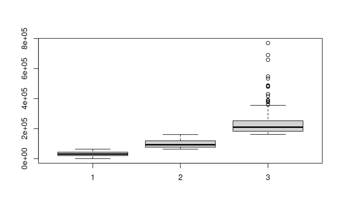
abc_ol <- which.min(bp$stats[3, ]) ## find out which group is A1, B1 overlapped
abc_nol <- which.max(bp$stats[3, ]) ## find out which group is A1, B1 not overlapped

## aggregate, this method only work for real 3D structure
#cg_xyz <- aggregateXYZs(xyz.list)
## get the cells which can represent the group
centers_cell <- getMedoidId(cd, cell_groups, N = 2)
centers_cell
## $`1`
## [1] "1114" "1843"
##
## $`2`
## [1] "234" "4311"
##
## $`3`
## [1] "1400" "3764"
cg_xyz <- xyz.s[unlist(centers_cell)]

## help function to get the coordinates in genome.
st <- function(i, offset=28000001, interval=30000){
  return(interval*i+offset)
}

## add genomic coordinates to XYZ matrix and make a GRanges object
cg_xyz <- lapply(cg_xyz, function(.ele){
  with(.ele, GRanges('chr21',
                     IRanges(st(.ele$Segment.index-1, offset=start(range)),
                             width = 30000),
                     x=X, y=Y, z=Z))
})


ABC <- GRanges('chr21', IRanges(st(c(18, 27, 32)-1, offset=start(range)), width = 30000),
               col=c('red', 'cyan', 'yellow'))
ABC$label <- c('A1', 'B1', 'C1')
ABC$type <- 'tad'
ABC$lwd <- 8
feature.gr$lwd <- 2
ABC.features <- c(feature.gr, ABC)

## visualize the grouped structures.
grouped_cell <- lapply(cg_xyz, function(cell){
  cell <- view3dStructure(cell, feature.gr=ABC.features,
                          genomicSigs = imr90_genomicSigs,
                          reverseGenomicSigs = FALSE,,
                          renderer = 'none', region = range,
                          show_coor=TRUE, lwd.backbone = 0.25,
                          lwd.gene = 0.5,
                          length.arrow = unit(0.1, "native"))
})

title <- c("A1,B1 overlap", "A1,B1 do not overlap")
showPairs(grouped_cell[[(abc_ol-1)*2+1]], grouped_cell[[(abc_nol-1)*2+1]],
          title = title,
          height = NULL)
showPairs(grouped_cell[[(abc_ol-1)*2+2]], grouped_cell[[(abc_nol-1)*2+2]],
          title = title,
          height = NULL)
present single cell 3D structure with TADs based on the point cluster
The data were from diffraction-limited experiments for IMR90 cells.
# Fig. S7
xyz <- read.csv('https://github.com/BogdanBintu/ChromatinImaging/raw/refs/heads/master/Data/IMR90_chr21-18-20Mb.csv', skip = 1)
xyz.s <- split(xyz[, -1], xyz$Chromosome.index)

#cd <- cellDistance(xyzs=lapply(xyz.s, function(.ele) fill_NA(.ele[, -1])), distance_method = 'NID',  eps = 'auto', rescale = FALSE)
cd <- readRDS(system.file('extdata', 'ChromatinImaging', 'FigS7.cellDistance.nid.rds', package = 'geomeTriD.documentation'))
cd1 <- as.matrix(cd)
cc1 <- apply(cd1[c(8, 9, 15, 26, 56), ], ## select some typical cells
             1, function(.ele){
  order(.ele)
})
cc <- cellClusters(cd)
#plot(cc, labels=FALSE)
cell_groups <- cutree(cc, h=0.5)

range_18_20 <- GRanges("chr21:18627683-20577682")
# feature.gr_18_20 <- getFeatureGR(txdb = TxDb.Hsapiens.UCSC.hg38.knownGene,
#                                  org = org.Hs.eg.db,
#                                  range = range_18_20)
## apply matlab.like2 colors for backbone
resolution <- 3
backbone_colors <- rev(matlab.like2(n=resolution*nrow(xyz.s[[1]])))

## help function to get the coordinates in genome.
st <- function(i, offset=28000001, interval=30000){
  return(interval*i+offset)
}

imr90_18_20 <- lapply(xyz.s, function(.ele){
  with(.ele, GRanges('chr21', IRanges(st(.ele$Segment.index-1,
                                         offset=start(range_18_20)),
                                      width = 30000),
                     x=X, y=Y, z=Z))
})

cells_18_20 <- list()
for(i in as.numeric(cc1[1:2, ])){
  try({
    cell <- imr90_18_20[[i]]
    cell <- cell[apply(mcols(cell), 1, function(.ele) !any(is.na(.ele)))]
    cell <- view3dStructure(cell, #feature.gr=feature.gr_18_20,
                            renderer = 'none', region = range_18_20,
                            show_coor=TRUE, lwd.backbone = 2,
                            col.backbone=backbone_colors,
                            resolution=resolution,
                            length.arrow = unit(0.1, "native"),
                            cluster3Dpoints = TRUE)
    ## reset the color for the point clusters
    pcn <- names(cell)[grepl('pointCluster', names(cell))]
    for(j in seq_along(pcn)){
      cell[[pcn[j]]]$colors <- j+1
    }
    cells_18_20[[i]] <- cell
  })
}

showPairs(cells_18_20[[cc1[1, '9']]], cells_18_20[[cc1[2, '9']]],
          height = NULL)# cell 1
showPairs(cells_18_20[[cc1[1, '56']]], cells_18_20[[cc1[2, '56']]],
          height = NULL)# cell 2
showPairs(cells_18_20[[cc1[1, '8']]], cells_18_20[[cc1[2, '8']]],
          height = NULL) # cell 3
showPairs(cells_18_20[[cc1[1, '26']]], cells_18_20[[cc1[2, '26']]],
          height = NULL)
SessionInfo
## R version 4.5.0 (2025-04-11)
## Platform: x86_64-pc-linux-gnu
## Running under: Ubuntu 24.04.2 LTS
##
## Matrix products: default
## BLAS:   /usr/lib/x86_64-linux-gnu/openblas-pthread/libblas.so.3
## LAPACK: /usr/lib/x86_64-linux-gnu/openblas-pthread/libopenblasp-r0.3.26.so;  LAPACK version 3.12.0
##
## locale:
##  [1] LC_CTYPE=en_US.UTF-8       LC_NUMERIC=C
##  [3] LC_TIME=en_US.UTF-8        LC_COLLATE=en_US.UTF-8
##  [5] LC_MONETARY=en_US.UTF-8    LC_MESSAGES=en_US.UTF-8
##  [7] LC_PAPER=en_US.UTF-8       LC_NAME=C
##  [9] LC_ADDRESS=C               LC_TELEPHONE=C
## [11] LC_MEASUREMENT=en_US.UTF-8 LC_IDENTIFICATION=C
##
## time zone: Etc/UTC
## tzcode source: system (glibc)
##
## attached base packages:
## [1] grid      stats4    stats     graphics  grDevices utils     datasets
## [8] methods   base
##
## other attached packages:
##  [1] colorRamps_2.3.4
##  [2] clusterCrit_1.3.0
##  [3] org.Hs.eg.db_3.21.0
##  [4] TxDb.Hsapiens.UCSC.hg38.knownGene_3.21.0
##  [5] GenomicFeatures_1.61.3
##  [6] AnnotationDbi_1.71.0
##  [7] Biobase_2.69.0
##  [8] GenomicRanges_1.61.0
##  [9] GenomeInfoDb_1.45.4
## [10] IRanges_2.43.0
## [11] S4Vectors_0.47.0
## [12] BiocGenerics_0.55.0
## [13] generics_0.1.4
## [14] geomeTriD.documentation_0.0.3
## [15] geomeTriD_1.3.11
##
## loaded via a namespace (and not attached):
##   [1] BiocIO_1.19.0               bitops_1.0-9
##   [3] filelock_1.0.3              tibble_3.3.0
##   [5] R.oo_1.27.1                 XML_3.99-0.18
##   [7] rpart_4.1.24                lifecycle_1.0.4
##   [9] httr2_1.1.2                 aricode_1.0.3
##  [11] globals_0.18.0              lattice_0.22-7
##  [13] ensembldb_2.33.0            MASS_7.3-65
##  [15] backports_1.5.0             magrittr_2.0.3
##  [17] Hmisc_5.2-3                 sass_0.4.10
##  [19] rmarkdown_2.29              jquerylib_0.1.4
##  [21] yaml_2.3.10                 plotrix_3.8-4
##  [23] Gviz_1.53.0                 DBI_1.2.3
##  [25] RColorBrewer_1.1-3          abind_1.4-8
##  [27] purrr_1.0.4                 R.utils_2.13.0
##  [29] AnnotationFilter_1.33.0     biovizBase_1.57.0
##  [31] RCurl_1.98-1.17             rgl_1.3.18
##  [33] nnet_7.3-20                 VariantAnnotation_1.55.0
##  [35] rappdirs_0.3.3              grImport_0.9-7
##  [37] listenv_0.9.1               parallelly_1.45.0
##  [39] pkgdown_2.1.3               codetools_0.2-20
##  [41] DelayedArray_0.35.1         xml2_1.3.8
##  [43] tidyselect_1.2.1            UCSC.utils_1.5.0
##  [45] farver_2.1.2                matrixStats_1.5.0
##  [47] BiocFileCache_2.99.5        base64enc_0.1-3
##  [49] GenomicAlignments_1.45.0    jsonlite_2.0.0
##  [51] trackViewer_1.45.0          progressr_0.15.1
##  [53] Formula_1.2-5               systemfonts_1.2.3
##  [55] dbscan_1.2.2                tools_4.5.0
##  [57] progress_1.2.3              ragg_1.4.0
##  [59] strawr_0.0.92               Rcpp_1.0.14
##  [61] glue_1.8.0                  gridExtra_2.3
##  [63] SparseArray_1.9.0           xfun_0.52
##  [65] MatrixGenerics_1.21.0       dplyr_1.1.4
##  [67] withr_3.0.2                 fastmap_1.2.0
##  [69] latticeExtra_0.6-30         rhdf5filters_1.21.0
##  [71] digest_0.6.37               R6_2.6.1
##  [73] textshaping_1.0.1           colorspace_2.1-1
##  [75] jpeg_0.1-11                 dichromat_2.0-0.1
##  [77] biomaRt_2.65.0              RSQLite_2.4.1
##  [79] R.methodsS3_1.8.2           data.table_1.17.4
##  [81] rtracklayer_1.69.0          prettyunits_1.2.0
##  [83] InteractionSet_1.37.0       httr_1.4.7
##  [85] htmlwidgets_1.6.4           S4Arrays_1.9.1
##  [87] pkgconfig_2.0.3             gtable_0.3.6
##  [89] blob_1.2.4                  XVector_0.49.0
##  [91] htmltools_0.5.8.1           ProtGenerics_1.41.0
##  [93] clue_0.3-66                 scales_1.4.0
##  [95] png_0.1-8                   knitr_1.50
##  [97] rstudioapi_0.17.1           rjson_0.2.23
##  [99] checkmate_2.3.2             curl_6.3.0
## [101] cachem_1.1.0                rhdf5_2.53.1
## [103] stringr_1.5.1               parallel_4.5.0
## [105] foreign_0.8-90              restfulr_0.0.15
## [107] desc_1.4.3                  pillar_1.10.2
## [109] vctrs_0.6.5                 RANN_2.6.2
## [111] dbplyr_2.5.0                cluster_2.1.8.1
## [113] htmlTable_2.4.3             evaluate_1.0.3
## [115] cli_3.6.5                   compiler_4.5.0
## [117] Rsamtools_2.25.0            rlang_1.1.6
## [119] crayon_1.5.3                future.apply_1.20.0
## [121] interp_1.1-6                fs_1.6.6
## [123] stringi_1.8.7               deldir_2.0-4
## [125] BiocParallel_1.43.3         txdbmaker_1.5.4
## [127] Biostrings_2.77.1           lazyeval_0.2.2
## [129] Matrix_1.7-3                BSgenome_1.77.0
## [131] hms_1.1.3                   bit64_4.6.0-1
## [133] future_1.58.0               ggplot2_3.5.2
## [135] Rhdf5lib_1.31.0             KEGGREST_1.49.0
## [137] SummarizedExperiment_1.39.0 igraph_2.1.4
## [139] memoise_2.0.1               bslib_0.9.0
## [141] bit_4.6.0