Figure 4 Vignette

Figure 4

Figure 4 showcases the capabilities of the geomeTriD package in visualizing data from STORM (Stochastic Optical Reconstruction Microscopy) and MERFISH (Multiplexed Error-Robust Fluorescence In Situ Hybridization). Since these methods provide real 3D spatial coordinates, the resulting point clouds can be clustered based on spatial distance. The spatial distance matrix can also be used to identify topologically associating domains (TADs) and compartments. In the context of single-cell 3D structures, this figure further demonstrates how geomeTriD can be used to cluster individual cells through analysis of their spatial distance matrices by multiple methods.

Load Libraries

library(geomeTriD)
library(geomeTriD.documentation)
library(GenomicRanges)
library(TxDb.Hsapiens.UCSC.hg38.knownGene)
#library(BSgenome.Hsapiens.UCSC.hg38)
library(org.Hs.eg.db)
library(colorRamps)
library(dendextend)
library(geometry)

Visualize single cell 3D structure for STROM data

The data are derived from diffraction-limited experiments for IMR90 cells. To demonstrate the capability of geomeTriD in visualizing multiple genomic signals along 3D structures, we incorporate bulk CTCF, SMC3, and RAD21 signal tracks. Cells are clustered based on their spatial similarity, using the Euclidean distance of each cell’s 3D structure to the centroid. Representative 3D structures from each cluster are then visualized.

## xyz is from diffraction-limited experiments but not the actual xyz cords of STORM experiments.
xyz <- read.csv('https://github.com/BogdanBintu/ChromatinImaging/raw/refs/heads/master/Data/IMR90_chr21-28-30Mb.csv', skip = 1)
## split the XYZ for each chromosome
xyz.s <- split(xyz[, -1], xyz$Chromosome.index)
head(xyz.s[[1]])

##   Segment.index    Z      X     Y
## 1             1 3090 135130 50097
## 2             2 3096 135094 50393
## 3             3 3216 135329 49882
## 4             4 3209 135166 50006
## 5             5 3153 135046 50028
## 6             6 3285 134862 49955

range <- GRanges("chr21:28000001-29200000")
### get feature annotations
feature.gr <- getFeatureGR(txdb = TxDb.Hsapiens.UCSC.hg38.knownGene,
                           org = org.Hs.eg.db,
                           range = range)

##   2169 genes were dropped because they have exons located on both strands of
##   the same reference sequence or on more than one reference sequence, so cannot
##   be represented by a single genomic range.
##   Use 'single.strand.genes.only=FALSE' to get all the genes in a GRangesList
##   object, or use suppressMessages() to suppress this message.

## 'select()' returned 1:1 mapping between keys and columns

### get genomic signals, we will use called peaks
colorSets <- c(CTCF="cyan",YY1="yellow",
               RAD21="red", SMC1A="green", SMC3="blue")
prefix <- 'https://www.encodeproject.org/files/'
imr90_url <- c(ctcf = 'ENCFF203SRF/@@download/ENCFF203SRF.bed.gz',
               smc3 = 'ENCFF770ISZ/@@download/ENCFF770ISZ.bed.gz',
               rad21 = 'ENCFF195CYT/@@download/ENCFF195CYT.bed.gz')
imr90_urls <- paste0(prefix, imr90_url)
names(imr90_urls) <- names(imr90_url)
# download the files and import the signals
imr90_genomicSigs <- importSignalFromUrl(imr90_urls, range = range,
                                         cols = list(
                                           'ctcf'=c('#111100', 'cyan'),
                                           'smc3'=c('#000011', 'blue'),
                                           'rad21'=c('#110000', 'red')),
                                         format = 'BED')

## adding rname 'https://www.encodeproject.org/files/ENCFF203SRF/@@download/ENCFF203SRF.bed.gz'

## Error while performing HEAD request.
##    Proceeding without cache information.

## adding rname 'https://www.encodeproject.org/files/ENCFF770ISZ/@@download/ENCFF770ISZ.bed.gz'

## Error while performing HEAD request.
##    Proceeding without cache information.

## adding rname 'https://www.encodeproject.org/files/ENCFF195CYT/@@download/ENCFF195CYT.bed.gz'

## Error while performing HEAD request.
##    Proceeding without cache information.

## select the interesting genomic regions for clustering cells
xyzs <- lapply(xyz.s, function(.ele) {
  .ele <- .ele[c(18, 27, 32), -1]
  if(any(is.na(.ele))) return(NULL)
  return(.ele)
})
keep <- lengths(xyzs)>0

## cluster the cells by distance of SDC
cd <- cellDistance(xyzs[keep], distance_method = 'DSDC')
cc <- cellClusters(cd)
cell_groups <- cutree(cc, k=3)

## check SDC (the mean of distance from each point to the centroid) for A1, B1, C1 
sdc <- sapply(xyzs[keep], SDC)
sdc <- split(sdc, cell_groups)
bp <- boxplot(sdc)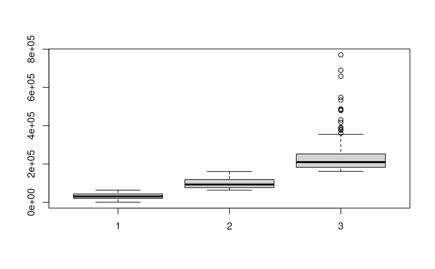

abc_ol <- which.min(bp$stats[3, ]) ## find out which group is A1, B1 overlapped
abc_nol <- which.max(bp$stats[3, ]) ## find out which group is A1, B1 not overlapped

## aggregate, this method only work for real 3D structure
#cg_xyz <- aggregateXYZs(xyz.list)
## get the cells which can represent the group
centers_cell <- getMedoidId(cd, cell_groups, N = 2)
centers_cell

## $`1`
## [1] "1114" "1843"
## 
## $`2`
## [1] "234"  "4311"
## 
## $`3`
## [1] "1400" "3764"

cg_xyz <- xyz.s[unlist(centers_cell)]

## help function to get the coordinates in genome.
st <- function(i, offset=28000001, interval=30000){
  return(interval*i+offset)
}

## add genomic coordinates to XYZ matrix and make a GRanges object
cg_xyz <- lapply(cg_xyz, function(.ele){
  with(.ele, GRanges('chr21',
                     IRanges(st(.ele$Segment.index-1, offset=start(range)),
                             width = 30000),
                     x=X, y=Y, z=Z))
})

## create a GRanges object for A1, B1, C1 
ABC <- GRanges('chr21', IRanges(st(c(18, 27, 32)-1,
                                   offset=start(range)),
                                width = 30000),
               col=c('red', 'cyan', 'yellow'))
ABC$label <- c('A1', 'B1', 'C1')
ABC$type <- 'tad'
ABC$lwd <- 8
feature.gr$lwd <- 2
ABC.features <- c(feature.gr, ABC)

## visualize the grouped structures.
grouped_cell <- lapply(cg_xyz, function(cell){
  cell <- view3dStructure(cell, feature.gr=ABC.features,
                          genomicSigs = imr90_genomicSigs,
                          reverseGenomicSigs = FALSE,,
                          renderer = 'none', region = range,
                          show_coor=TRUE, lwd.backbone = 0.25,
                          lwd.gene = 0.5,
                          length.arrow = unit(0.1, "native"))
})

title <- c("A1,B1 overlap", "A1,B1 do not overlap")
showPairs(grouped_cell[[(abc_ol-1)*2+1]], grouped_cell[[(abc_nol-1)*2+1]],
          title = title)

showPairs(grouped_cell[[(abc_ol-1)*2+2]], grouped_cell[[(abc_nol-1)*2+2]],
          title = title)

Visualize single cell 3D structure with point clouds

The data originate from diffraction-limited experiments for IMR90 cells, specifically targeting the 18–20 Mb region of chromosome 21. Here, we present single-cell 3D structures with spatial point clusters identified using DBSCAN. In addition, we display the corresponding spatial distance matrices as heatmaps, annotated with predicted TADs, compartments, and point cloud boundaries, to highlight the structural organization of this genomic region.

## the raw data are same as the Fig. S7 from the original paper
xyz <- read.csv('https://github.com/BogdanBintu/ChromatinImaging/raw/refs/heads/master/Data/IMR90_chr21-18-20Mb.csv', skip = 1)
xyz.s <- split(xyz[, -1], xyz$Chromosome.index)

## get cell distance matrix by Normalized information distance (NID) for the point clouds using DBSCAN 
#cd <- cellDistance(xyzs=lapply(xyz.s, function(.ele) fill_NA(.ele[, -1])), distance_method = 'NID',  eps = 'auto', rescale = FALSE)
## we load pre-calculated data
cd <- readRDS(system.file('extdata', 'ChromatinImaging', 'FigS7.cellDistance.nid.rds', package = 'geomeTriD.documentation'))
cd1 <- as.matrix(cd)
cc1 <- apply(cd1[c(8, 9, 15, 26, 56), ], ## select some typical cells
             1, function(.ele){
  order(.ele)
})

range_18_20 <- GRanges("chr21:18627683-20577682")
# feature.gr_18_20 <- getFeatureGR(txdb = TxDb.Hsapiens.UCSC.hg38.knownGene,
#                                  org = org.Hs.eg.db,
#                                  range = range_18_20)
## apply matlab.like2 colors for backbone
resolution <- 3
backbone_colors <- rev(matlab.like2(n=resolution*nrow(xyz.s[[1]])))

## help function to get the coordinates in genome.
st <- function(i, offset=28000001, interval=30000){
  return(interval*i+offset)
}

## create the GRanges object with x, y, z coordinates
imr90_18_20 <- lapply(xyz.s, function(.ele){
  with(.ele, GRanges('chr21', IRanges(st(.ele$Segment.index-1,
                                         offset=start(range_18_20)),
                                      width = 30000),
                     x=X, y=Y, z=Z))
})

## create the threejsGeometry objects
cells_18_20 <- list()
for(i in as.numeric(cc1[1:2, ])){ ## find the nearest neighbor of selected cells
  try({
    cell <- imr90_18_20[[i]]
    cell <- cell[apply(mcols(cell), 1, function(.ele) !any(is.na(.ele)))]
    cell <- view3dStructure(cell, #feature.gr=feature.gr_18_20,
                            renderer = 'none', region = range_18_20,
                            show_coor=TRUE, lwd.backbone = 2,
                            col.backbone=backbone_colors,
                            resolution=resolution,
                            length.arrow = unit(0.1, "native"),
                            cluster3Dpoints = TRUE)
    ## reset the color for the point clouds
    pcn <- names(cell)[grepl('pointCluster', names(cell))]
    for(j in seq_along(pcn)){
      cell[[pcn[j]]]$colors <- j+1
    }
    cells_18_20[[i]] <- cell
  })
}
## help function to show the spatical distance matrix, 
## the TADs, compartments and the point clusters boundaries.
plotdistance <- function(xyz){
  pc <- pointCluster(fill_NA(xyz))
  spatialDistanceHeatmap(xyz,
                         col=colorRampPalette(c("#871518", "#FF0000",
                                                "#FFFFFF", "#00008B",
                                                '#20205F'))(100),
                         components = c('compartment'))
  ## use green color line to present the point cluster boundaries.
  pid <- unique(pc$cluster)
  for(id in pid){
    if(id!=0){
      borders <- (range(which(pc$cluster==id))+c(-.5, .5))/length(pc$cluster)
      rect(xleft = borders[1], ybottom = (0.985-borders[2])*10/11.5,
           xright = borders[2], ytop = (0.985-borders[1])*10/11.5,
           col = NA, border = 'green', lwd = 2)
    }
  }
}

showPairs(cells_18_20[[cc1[1, '9']]], cells_18_20[[cc1[2, '9']]])# cell 1

plotdistance(imr90_18_20[[cc1[1, '9']]])

## eps is set to 160.911716095807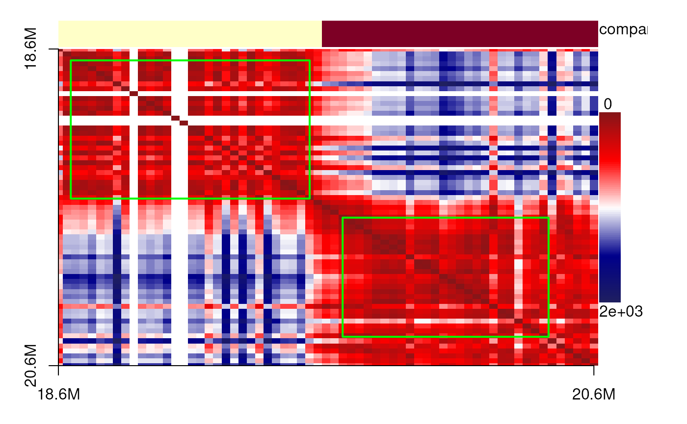

showPairs(cells_18_20[[cc1[1, '56']]], cells_18_20[[cc1[2, '56']]])# cell 2

plotdistance(imr90_18_20[[cc1[1, '56']]])

## eps is set to 255.85875256654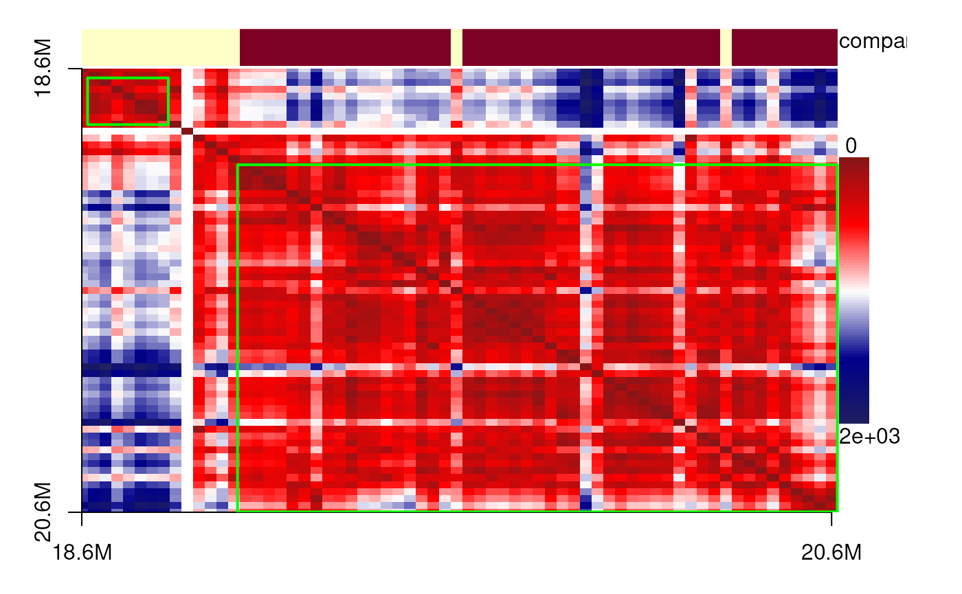

showPairs(cells_18_20[[cc1[1, '8']]], cells_18_20[[cc1[2, '8']]]) # cell 3

plotdistance(imr90_18_20[[cc1[1, '8']]])

## eps is set to 239.124324562482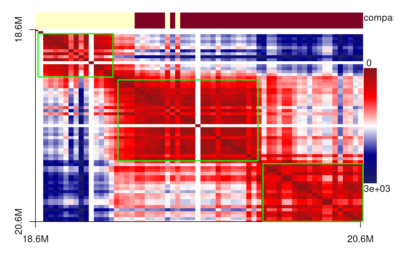

showPairs(cells_18_20[[cc1[1, '26']]], cells_18_20[[cc1[2, '26']]])

plotdistance(imr90_18_20[[cc1[1, '26']]])

## eps is set to 70.9963426614948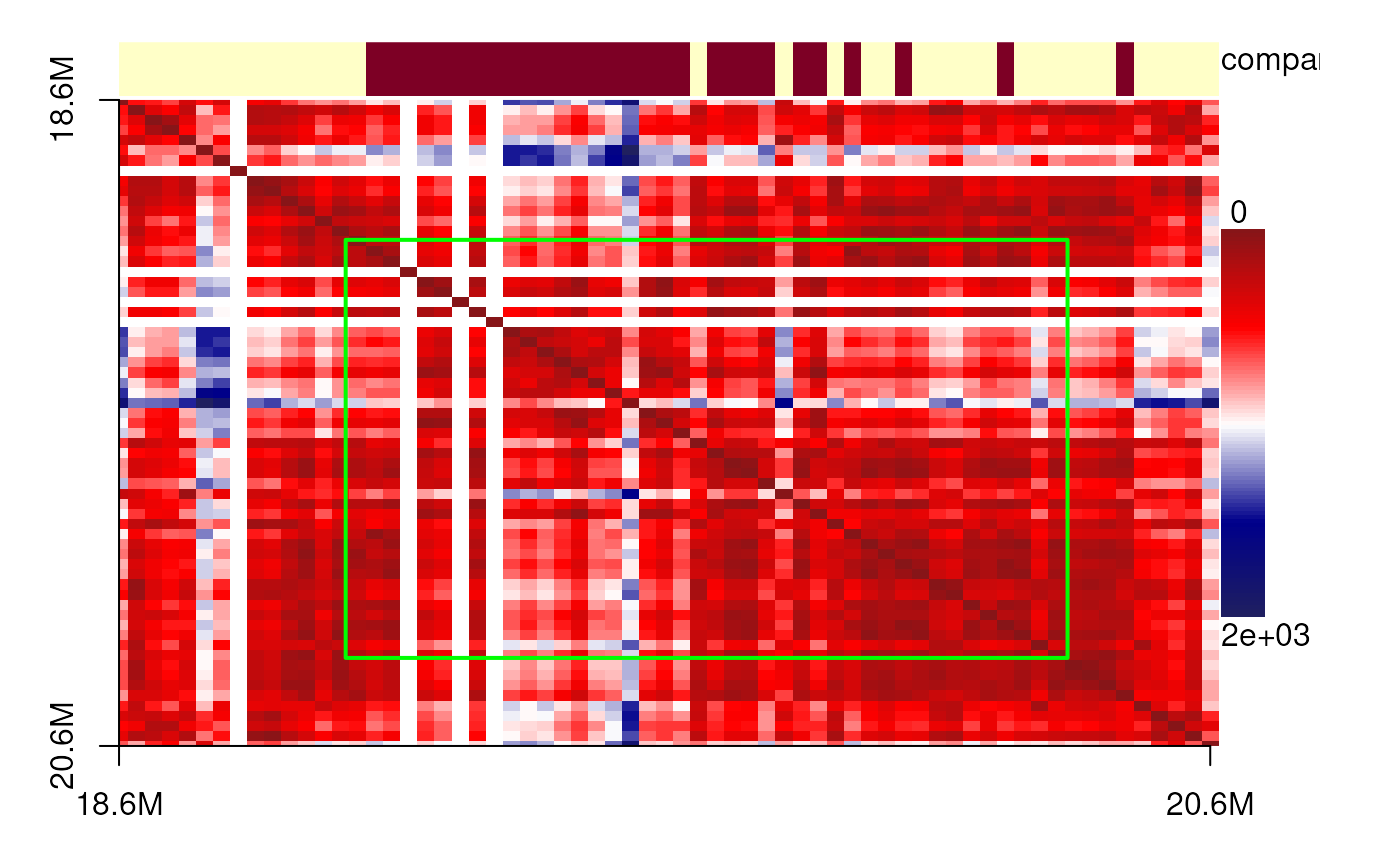

## check the size 
getV <- function(i){
  vol <- convhulln(as.matrix(mcols(fill_NA(imr90_18_20[[i]]))), options='Fa')$vol
}
sapply(cc1[1, c('9', '56', '8', '26')], getV)

##          9         56          8         26 
##  435730383  680580453 1120495581  300372003

Visualize single cell 3D structure for MERFISH data

The data were obtained from a MERFISH-based 3D chromatin study of chromosome 21 in IMR90 cells. We first cluster the cells based on their spatial features, then select representative cells from each cluster. For these cells, we visualize the spatial distance matrices as heatmaps and display their corresponding 3D genome structures annotated with predicted TADs and compartments.

# chr21 <- read.delim('.../MERFISH/chromosome21.tsv')
# chr21 <- with(chr21, GRanges(Genomic.coordinate,
#                              x=X.nm., y=Y.nm., z=Z.nm.,
#                              cell=Chromosome.copy.number))
# chr21 <- split(chr21, chr21$cell)
# chr21 <- lapply(chr21, function(.ele){
#   .ele$cell <- NULL
#   .ele
# })
# cd <- cellDistance(xyzs=lapply(chr21[1:1000], function(.ele) fill_NA(as.data.frame(mcols(.ele)))), distance_method = 'NID', k = 'auto')
extdata <- system.file('extdata', 'MERFISH', package = 'geomeTriD.documentation')
chr21 <- readRDS(file.path(extdata, 'chromosome21.1K.cell.rds'))
cd <- readRDS(file.path(extdata, 'celldist.NID.rds'))
cc <- cellClusters(cd)
k <- autoK(cd, cc, max_k = 10)
cell_groups <- cutree(cc, k=k)
centers_cell <- getMedoidId(cd, cell_groups)
## plot the select cells
dend <- as.dendrogram(cc)
labels(dend) <- ifelse(labels(dend) %in% unlist(centers_cell), labels(dend), '')
plot(dend)

## Cluster the selected cells into pairs for comparative visualization.
cd1 <- cellDistance(lapply(chr21[unlist(centers_cell)], function(.ele) fill_NA(as.data.frame(mcols(.ele)))), distance_method = 'NID', k='auto')
cc1 <- cellClusters(cd1)
plot(cc1)

## plot the spatial distance matrix
plotSDM <- function(gr, cutoff=1500, components=c('compartment'), ...){
  sdm <- spatialDistanceMatrix(gr)
  sdm[sdm>cutoff] <- cutoff ## this is used to remove the outliers
  spatialDistanceHeatmap(sdm,
                         components = components,
                         col=colorRampPalette(c("#871518", "#FF0000",
                                                "#FFFFFF", "#00008B",
                                                '#20205F'))(100),
                         Gaussian_blur = TRUE,
                         ...)
}
plotSDM(chr21[[centers_cell[[1]]]])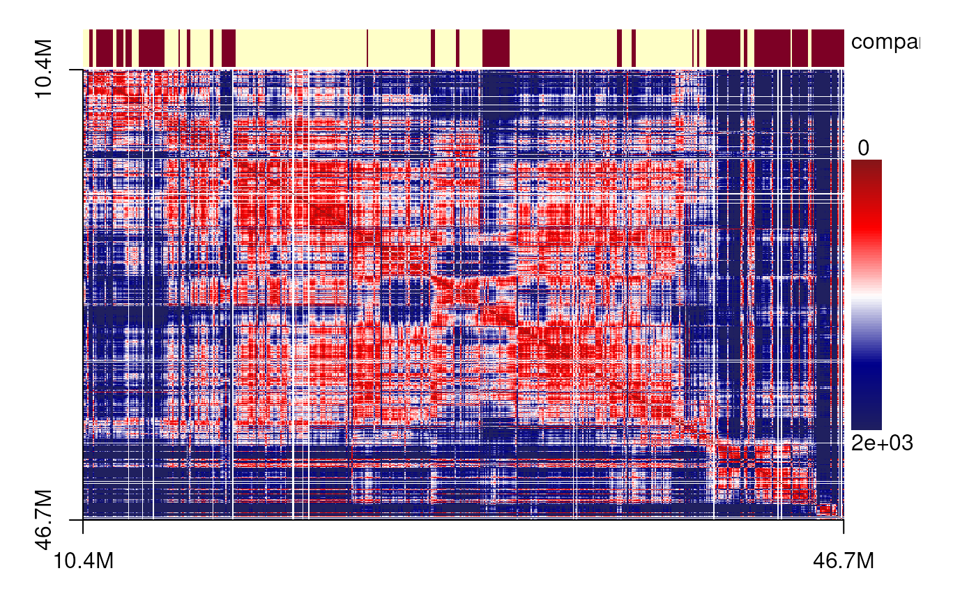

plotSDM(chr21[[centers_cell[[2]]]])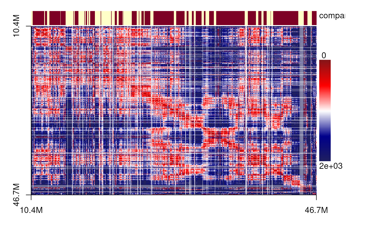

plotSDM(chr21[[centers_cell[[3]]]])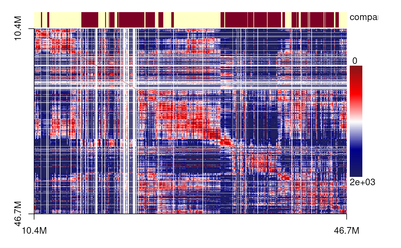

plotSDM(chr21[[centers_cell[[5]]]])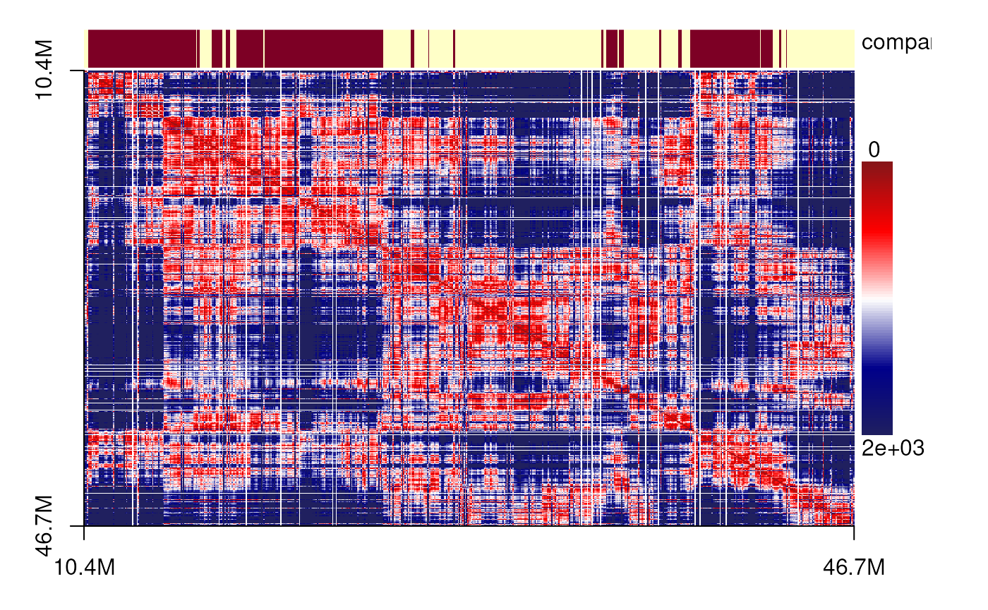

plotSDM(chr21[[centers_cell[[4]]]])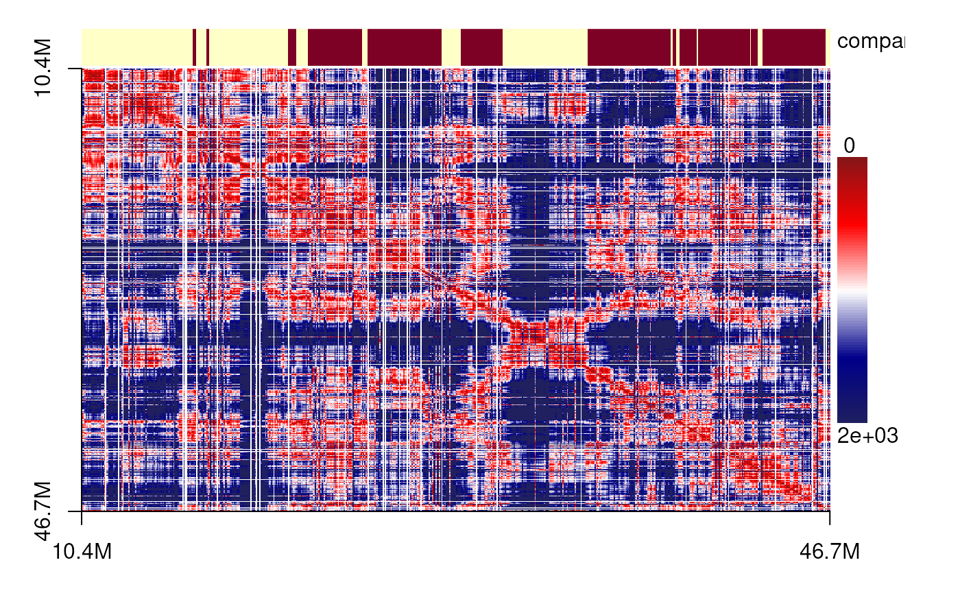

plotSDM(chr21[[centers_cell[[6]]]])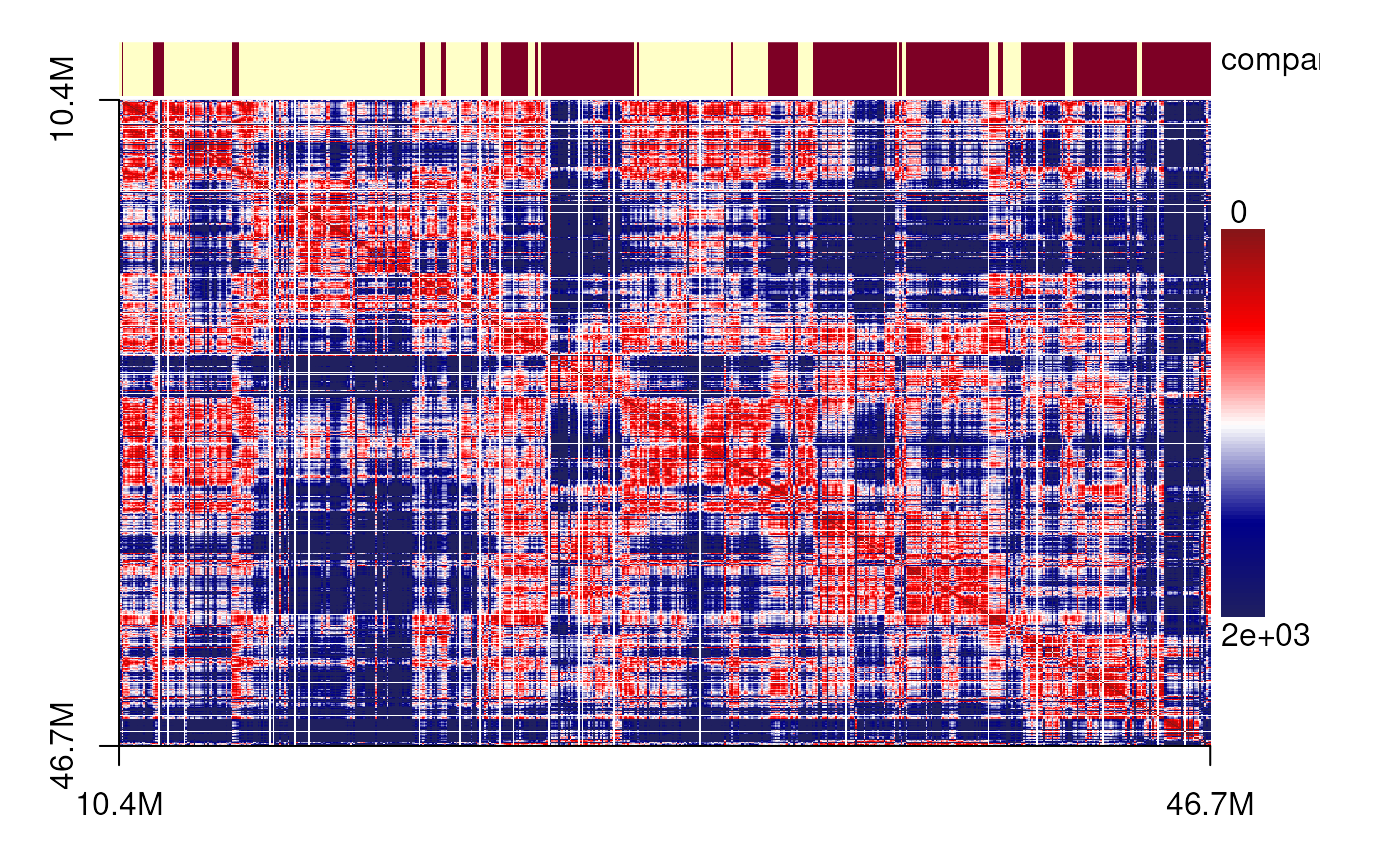

resolution <- 3
backbone_colors <- rev(matlab.like2(n=resolution*length(chr21[[1]])))

MERFISH_cells <- lapply(unlist(centers_cell), function(i){
  cell <- chr21[[i]]
  sdm <- spatialDistanceMatrix(cell)
  sdm <- gaussianBlur(sdm) ## do Gaussian blur to reduce the noise
  ## get the TADs by hierarchical clustering method
  tads <- hierarchicalClusteringTAD(sdm, bin_size=width(cell)[1])
  tads <- apply(tads, 1, function(.ele){
    range(cell[seq(.ele[1], .ele[2])])
  })
  tads <- unlist(GRangesList(tads))
  ## get the compartments
  ## The genome is used to adjust A/B by GC contents.
  ## It is highly suggested for real data.
  compartments <- compartment(cell)#, genome = BSgenome.Hsapiens.UCSC.hg38)
  ## create the threejsGeometry object
  cell <- cell[apply(mcols(cell), 1, function(.ele) !any(is.na(.ele)))]
  cell <- view3dStructure(cell, feature.gr = compartments,
                          renderer = 'none',
                          show_coor=FALSE, lwd.backbone = 2,
                          col.backbone=backbone_colors,
                          resolution=resolution,
                          length.arrow = unit(0.1, "native"))
  ## add TADs as segments
  backbone <- extractBackbonePositions(cell)
  tads <- createTADGeometries(tads, backbone, type = 'segment', lwd=4, alpha = 0.5)
  c(cell, tads)
})


showPairs(MERFISH_cells[[1]], MERFISH_cells[[2]])

showPairs(MERFISH_cells[[4]], MERFISH_cells[[6]])

showPairs(MERFISH_cells[[3]], MERFISH_cells[[5]])

SessionInfo

sessionInfo()