Figure S4 HiRES
Figure S4 HiRES showcases the geomeTriD package,
demonstrating how it presents 3D models along with multiple genomic
signals mapped onto single-cell 3D structures.
Present single cell 3D structure for HiRES data
This dataset was generated using HiRES, an assay that
stands for “Hi-C and RNA-seq employed simultaneously.” HiRES enables the
simultaneous profiling of single-cell Hi-C and RNA-seq data. The
resulting Hi-C data can be used to predict 3D genome structures using
Dip-C, and the corresponding RNA-seq data can be visualized
along these structures using the geomeTriD package.
## load data for HiRES
extdata <- system.file('extdata', 'GSE223917', package = 'geomeTriD.documentation')
HiRES <- readRDS(file.path(extdata, 'HiRES.radial_glias.G1.chrX.rds')) # Dip-C predicted 3D structure
exprs <- readRDS(file.path(extdata, 'expr.radial_glias.G1.chrX.rds'))# RNA-seq data
pairs <- readRDS(file.path(extdata, 'sel.imput.pairs.chrX.rds')) # selected impute pairs
### supperloop
supperloops <- GRanges(c('chrX:50555744-50635321',
'chrX:75725458-75764699', # 4933407K13RiK, NR_029443
'chrX:103422010-103484957',
'chrX:105040854-105117090')) # 5530601H04RiK, NR_015467 and Pbdc1
names(supperloops) <- c('Firre', 'Dxz4', 'Xist/Tsix', 'x75')
supperloops$label <- names(supperloops)
supperloops$col <- 2:5 ## set colors for each element
supperloops$type <- 'gene' ## set it as gene
## plot region
range <- as(seqinfo(TxDb.Mmusculus.UCSC.mm10.knownGene)['chrX'], 'GRanges')
## annotations
genes <- genes(TxDb.Mmusculus.UCSC.mm10.knownGene)## 66 genes were dropped because they have exons located on both strands of the
## same reference sequence or on more than one reference sequence, so cannot be
## represented by a single genomic range.
## Use 'single.strand.genes.only=FALSE' to get all the genes in a GRangesList
## object, or use suppressMessages() to suppress this message.
genes_symbols <- mget(genes$gene_id, org.Mm.egSYMBOL, ifnotfound = NA)
genes$symbols <- sapply(genes_symbols, `[`, i=1)
geneX <- genes[seqnames(genes)=='chrX']
geneX$label <- geneX$symbols
geneX <- geneX[geneX$symbols %in% rownames(exprs)]
## get data for female, must have mat and pat info for chromosome X.
HiRES.mat <- lapply(HiRES, function(.ele) {
.ele <- .ele[.ele$parental=='(mat)']
.ele$parental <- NULL
.ele
})
HiRES.pat <- lapply(HiRES, function(.ele) {
.ele <- .ele[.ele$parental=='(pat)']
.ele$parental <- NULL
.ele
})
## remove the cells without chrX structures
l.mat <- lengths(HiRES.mat)
l.pat <- lengths(HiRES.pat)
k <- l.mat>0 & l.pat>0
HiRES.mat <- HiRES.mat[k]
HiRES.pat <- HiRES.pat[k]
# Make all GRanges object in a list same length by filling with NA
HiRES <- paddingGRangesList(c(HiRES.mat, HiRES.pat))
HiRES.mat.xyzs <- HiRES$xyzs[seq_along(HiRES.mat)]
HiRES.pat.xyzs <- HiRES$xyzs[-seq_along(HiRES.mat)]
## prepare the maternal and paternal GRanges object with x, y, z coordinates.
HiRES.mat <- lapply(HiRES.mat.xyzs, function(.ele){
gr <- HiRES$gr
mcols(gr) <- .ele[, c('x', 'y', 'z')]
gr
})
HiRES.pat <- lapply(HiRES.pat.xyzs, function(.ele){
gr <- HiRES$gr
mcols(gr) <- .ele[, c('x', 'y', 'z')]
gr
})
## backbone color
resolution <- 3
backbone_colors <- matlab.like2(n=resolution*length(HiRES.mat[[1]]))
backbone_bws <- backbone_colors ## defines the color assigned to the chrX allele
backbone_bws[1001:(length(backbone_colors)-1000)] <- 'gray'
## help function to check the volume of the 3D structure
getV <- function(points){
vol <- convhulln(points, options='Fa')$vol
}
## calculate the Root Mean Square Deviation (RMSD)
RMSD_mat_pat <- mapply(function(mat, pat){
mat <- as.data.frame(mcols(mat))
pat <- as.data.frame(mcols(pat))
mat <- fill_NA(mat)
pat <- fill_NA(pat)
pat <- alignCoor(pat, mat) # do alignment first
## normalized to its centroid
mat.center <- colMeans(mat, na.rm = TRUE)
pat.center <- colMeans(pat, na.rm = TRUE)
mat <- t(t(mat) - mat.center)
pat <- t(t(pat) - pat.center)
mean(sqrt(rowSums((mat - pat)^2)), na.rm = TRUE)
}, HiRES.mat, HiRES.pat)
## data frame for Xist expression level, total expression level and
## the RMSD between mat and pat
XlinkExpr <- data.frame(Xist=exprs['Xist', ], total=colSums(exprs), RMSD=RMSD_mat_pat)
XlinkExpr <- XlinkExpr[order(XlinkExpr$total), ]
## plot the correlation between RMSD and total chrX expression level
fit <- lm(RMSD ~ total, data = XlinkExpr)
plot(XlinkExpr$total, XlinkExpr$RMSD,
xlab='Total expression level of X-lined gene',
ylab='RMSD between maternal and paternal')
abline(fit, col = "blue", lwd=2)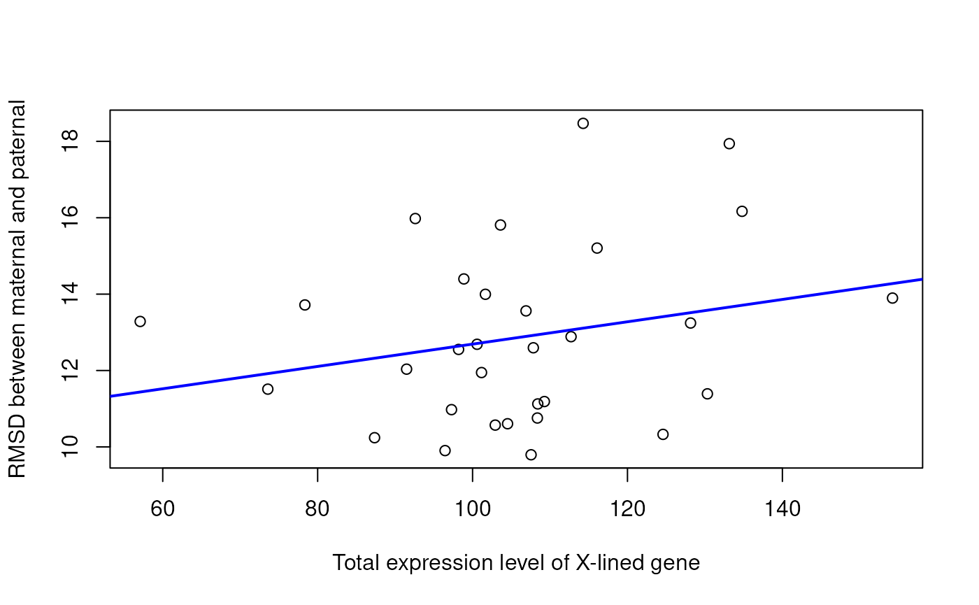
widgets <- lapply(c(head(rownames(XlinkExpr), n=2),
tail(rownames(XlinkExpr), n=2)), function(cell_id){
## expressions in single cell
exprSig <- geneX
exprSig$score <- exprs[geneX$symbols, cell_id]
## load the 3D structure for maternal and paternal
mat_cell <- HiRES.mat[[cell_id]]
mcols(mat_cell) <- fill_NA(as.data.frame(mcols(mat_cell)))
pat_cell <- HiRES.pat[[cell_id]]
mcols(pat_cell) <- fill_NA(as.data.frame(mcols(pat_cell)))
## check the volumn of the chrX,
## bigger one is Xa
## condensed one is Xi
v_mat <- getV(as.matrix(mcols(mat_cell)))
v_pat <- getV(as.matrix(mcols(pat_cell)))
## add additional information,
## Here we use the selected interactions by impute phases for maternal
mat_only_pairs <- pairs$mat[[cell_id]]
mat_only_pairs$color <- 'black'
mat_only_pairs$lwd <- 4
mat_cell <- view3dStructure(mat_cell,
feature.gr=supperloops,
lwd.gene = 4,
renderer = 'none',
region = range,
resolution=resolution,
genomicSigs = if(v_mat>v_pat) {
list(mat_rna_reads=exprSig, mat_pairs=mat_only_pairs)
} else {list(mat_pairs=mat_only_pairs)},
signalTransformFun = c,
reverseGenomicSigs = FALSE,
show_coor=FALSE,
lwd.backbone = 0.25,
col.backbone = if(v_mat>v_pat) backbone_bws else backbone_colors)
## and paternal only interactions by impute phases
pat_only_pairs <- pairs$pat[[cell_id]]
pat_only_pairs$color <- 'black'
pat_only_pairs$lwd <- 4
pat_cell <- view3dStructure(pat_cell,
feature.gr=supperloops,
lwd.gene = 4,
renderer = 'none',
region = range,
resolution=resolution,
genomicSigs = if(v_mat<=v_pat) {
list(pat_rna_reads=exprSig, pat_pairs=pat_only_pairs)
} else {list(pat_pairs=pat_only_pairs)},
signalTransformFun = c,
reverseGenomicSigs = FALSE,
show_coor=FALSE,
lwd.backbone = 0.25,
col.backbone = if(v_mat>v_pat) backbone_colors else backbone_bws)
# widget <-showPairs(mat_cell, pat_cell, title = paste(c('mat', 'pat'), cell_id))
# tempfile <- paste0('cell.', cell_id, '.html')
# htmlwidgets::saveWidget(widget, file=tempfile, selfcontained = FALSE, libdir = 'js')
showPairs(mat_cell, pat_cell,
title = paste(c('mat', 'pat'), cell_id),
height=NULL)
})
## low expression of X-linked genes
widgets[[1]]
#widgets[[2]]
## high expression of X-linked genes
#widgets[[3]]
widgets[[4]]SessionInfo
## R version 4.5.2 (2025-10-31)
## Platform: x86_64-pc-linux-gnu
## Running under: Ubuntu 24.04.3 LTS
##
## Matrix products: default
## BLAS: /usr/lib/x86_64-linux-gnu/openblas-pthread/libblas.so.3
## LAPACK: /usr/lib/x86_64-linux-gnu/openblas-pthread/libopenblasp-r0.3.26.so; LAPACK version 3.12.0
##
## locale:
## [1] LC_CTYPE=en_US.UTF-8 LC_NUMERIC=C
## [3] LC_TIME=en_US.UTF-8 LC_COLLATE=en_US.UTF-8
## [5] LC_MONETARY=en_US.UTF-8 LC_MESSAGES=en_US.UTF-8
## [7] LC_PAPER=en_US.UTF-8 LC_NAME=C
## [9] LC_ADDRESS=C LC_TELEPHONE=C
## [11] LC_MEASUREMENT=en_US.UTF-8 LC_IDENTIFICATION=C
##
## time zone: Etc/UTC
## tzcode source: system (glibc)
##
## attached base packages:
## [1] grid stats4 stats graphics grDevices utils datasets
## [8] methods base
##
## other attached packages:
## [1] geometry_0.5.2
## [2] org.Mm.eg.db_3.22.0
## [3] TxDb.Mmusculus.UCSC.mm10.knownGene_3.10.0
## [4] GenomicFeatures_1.62.0
## [5] AnnotationDbi_1.72.0
## [6] Biobase_2.70.0
## [7] colorRamps_2.3.4
## [8] GenomicRanges_1.62.0
## [9] Seqinfo_1.0.0
## [10] IRanges_2.44.0
## [11] S4Vectors_0.48.0
## [12] BiocGenerics_0.56.0
## [13] generics_0.1.4
## [14] geomeTriD.documentation_0.0.6
## [15] geomeTriD_1.5.0
##
## loaded via a namespace (and not attached):
## [1] BiocIO_1.20.0 bitops_1.0-9
## [3] filelock_1.0.3 tibble_3.3.0
## [5] R.oo_1.27.1 XML_3.99-0.20
## [7] rpart_4.1.24 lifecycle_1.0.4
## [9] httr2_1.2.1 aricode_1.0.3
## [11] globals_0.18.0 lattice_0.22-7
## [13] ensembldb_2.34.0 MASS_7.3-65
## [15] backports_1.5.0 magrittr_2.0.4
## [17] Hmisc_5.2-4 sass_0.4.10
## [19] rmarkdown_2.30 jquerylib_0.1.4
## [21] yaml_2.3.10 plotrix_3.8-4
## [23] Gviz_1.54.0 DBI_1.2.3
## [25] RColorBrewer_1.1-3 abind_1.4-8
## [27] R.utils_2.13.0 AnnotationFilter_1.34.0
## [29] biovizBase_1.58.0 RCurl_1.98-1.17
## [31] rgl_1.3.24 nnet_7.3-20
## [33] VariantAnnotation_1.56.0 rappdirs_0.3.3
## [35] grImport_0.9-7 listenv_0.10.0
## [37] parallelly_1.45.1 pkgdown_2.2.0
## [39] codetools_0.2-20 DelayedArray_0.36.0
## [41] tidyselect_1.2.1 UCSC.utils_1.6.0
## [43] farver_2.1.2 matrixStats_1.5.0
## [45] BiocFileCache_3.0.0 base64enc_0.1-3
## [47] GenomicAlignments_1.46.0 jsonlite_2.0.0
## [49] trackViewer_1.47.0 progressr_0.18.0
## [51] Formula_1.2-5 systemfonts_1.3.1
## [53] dbscan_1.2.3 tools_4.5.2
## [55] progress_1.2.3 ragg_1.5.0
## [57] strawr_0.0.92 Rcpp_1.1.0
## [59] glue_1.8.0 gridExtra_2.3
## [61] SparseArray_1.10.1 xfun_0.54
## [63] MatrixGenerics_1.22.0 GenomeInfoDb_1.46.0
## [65] dplyr_1.1.4 fastmap_1.2.0
## [67] latticeExtra_0.6-31 rhdf5filters_1.22.0
## [69] digest_0.6.38 R6_2.6.1
## [71] textshaping_1.0.4 colorspace_2.1-2
## [73] jpeg_0.1-11 dichromat_2.0-0.1
## [75] biomaRt_2.66.0 RSQLite_2.4.4
## [77] cigarillo_1.0.0 R.methodsS3_1.8.2
## [79] data.table_1.17.8 rtracklayer_1.70.0
## [81] prettyunits_1.2.0 InteractionSet_1.38.0
## [83] httr_1.4.7 htmlwidgets_1.6.4
## [85] S4Arrays_1.10.0 pkgconfig_2.0.3
## [87] gtable_0.3.6 blob_1.2.4
## [89] S7_0.2.0 XVector_0.50.0
## [91] htmltools_0.5.8.1 ProtGenerics_1.42.0
## [93] clue_0.3-66 scales_1.4.0
## [95] png_0.1-8 knitr_1.50
## [97] rstudioapi_0.17.1 rjson_0.2.23
## [99] magic_1.6-1 checkmate_2.3.3
## [101] curl_7.0.0 cachem_1.1.0
## [103] rhdf5_2.54.0 stringr_1.6.0
## [105] parallel_4.5.2 foreign_0.8-90
## [107] restfulr_0.0.16 desc_1.4.3
## [109] pillar_1.11.1 vctrs_0.6.5
## [111] RANN_2.6.2 dbplyr_2.5.1
## [113] cluster_2.1.8.1 htmlTable_2.4.3
## [115] evaluate_1.0.5 cli_3.6.5
## [117] compiler_4.5.2 Rsamtools_2.26.0
## [119] rlang_1.1.6 crayon_1.5.3
## [121] future.apply_1.20.0 interp_1.1-6
## [123] fs_1.6.6 stringi_1.8.7
## [125] deldir_2.0-4 BiocParallel_1.44.0
## [127] txdbmaker_1.6.0 Biostrings_2.78.0
## [129] lazyeval_0.2.2 Matrix_1.7-4
## [131] BSgenome_1.78.0 hms_1.1.4
## [133] bit64_4.6.0-1 future_1.67.0
## [135] ggplot2_4.0.0 Rhdf5lib_1.32.0
## [137] KEGGREST_1.50.0 SummarizedExperiment_1.40.0
## [139] igraph_2.2.1 memoise_2.0.1
## [141] bslib_0.9.0 bit_4.6.0