trackViewer Vignette: plot interaction data
Jianhong Ou, Lihua Julie Zhu
5 September 2024
plotInteractionData.RmdAbstract
Visualize chromatin interactions along with annotation as track layers. The interactions can be compared by back to back heatmaps. The interactions can be plot as heatmap and links.
Introduction
The chromatin interactions is involved in precise quantitative and spatiotemporal control of gene expression. The development of high-throughput experimental techniques, such as HiC-seq, HiCAR-seq, and InTAC-seq, for analyzing both the higher-order structure of chromatin and the interactions between protein and their nearby and remote regulatory elements has been developed to reveal how gene expression is controlled in genome-wide.
The interaction data will be saved in the format of paired genome
coordinates with the interaction score. The popular format are
.validPairs, .hic, and .cool. The
trackViewer package can be used to handle those data to
plot the heatmap or the interaction links.
Plot chromatin interactions data in linear layout
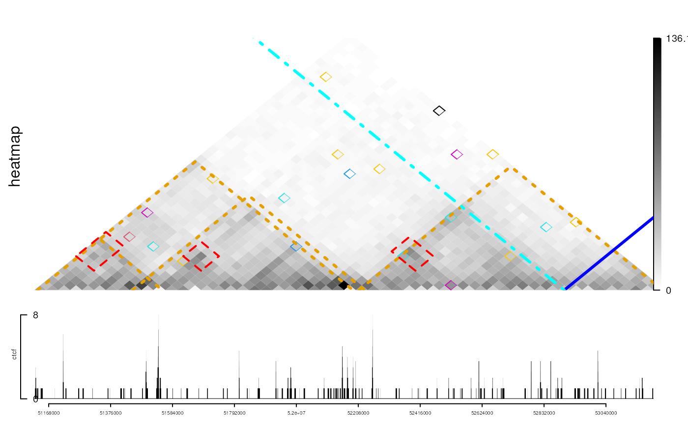
Plot chromatin interactions tracks as heatmap.
library(trackViewer)
library(InteractionSet)
gi <- readRDS(system.file("extdata", "nij.chr6.51120000.53200000.gi.rds", package="trackViewer"))
head(gi)
## GInteractions object with 6 interactions and 1 metadata column:
## seqnames1 ranges1 seqnames2 ranges2 | score
## <Rle> <IRanges> <Rle> <IRanges> | <numeric>
## [1] chr6 51120000-51160000 --- chr6 51120000-51160000 | 45.1227
## [2] chr6 51120000-51160000 --- chr6 51160000-51200000 | 35.0006
## [3] chr6 51120000-51160000 --- chr6 51200000-51240000 | 44.7322
## [4] chr6 51120000-51160000 --- chr6 51240000-51280000 | 29.3507
## [5] chr6 51120000-51160000 --- chr6 51280000-51320000 | 38.8417
## [6] chr6 51120000-51160000 --- chr6 51320000-51360000 | 31.7063
## -------
## regions: 53 ranges and 0 metadata columns
## seqinfo: 1 sequence from an unspecified genome; no seqlengths
## hicexplorer:hicConvertFormat tool can be used to convert other formats into GInteractions
## eg: hicConvertFormat -m mESC_rep.hic --inputFormat hic --outputFormat cool -o mESC_rep.mcool
##     hicConvertFormat -m mESC_rep.mcool::resolutions/10000 --inputFormat cool --outputFormat ginteractions -o mESC_rep.ginteractions --resolutions 10000
## please note that metadata:score is used for plot.
gi$border_color <- NA ## highlight some regions
gi$border_color[sample(seq_along(gi), 20)] <- sample(1:7, 20, replace=TRUE)
## The TADs will be drawn as lines at points start(first), center point, end(second).
tads <- GInteractions(
  GRanges("chr6",
          IRanges(c(51130001, 51130001, 51450001, 52210001), width = 20000)),
  GRanges("chr6",
          IRanges(c(51530001, 52170001, 52210001, 53210001), width = 20000)))
range <- GRanges("chr6", IRanges(51120000, 53200000))
heatmap <- gi2track(gi)
ctcf <- readRDS(system.file("extdata", "ctcf.sample.rds", package="trackViewer"))
viewTracks(trackList(ctcf, heatmap, heightDist = c(1, 3)),
           gr=range, autoOptimizeStyle = TRUE)
## add TAD information
addInteractionAnnotation(tads, "heatmap", grid.lines, gp=gpar(col="#E69F00", lwd=3, lty=3))
## add highlight interested regions
gi_sub <- gi[order(gi$score, decreasing = TRUE)]
gi_sub <- head(gi_sub[distance(first(gi_sub), second(gi_sub))>200000], n=5)
start(regions(gi_sub)) <- start(regions(gi_sub))-40000
end(regions(gi_sub)) <- end(regions(gi_sub))+40000
addInteractionAnnotation(gi_sub, "heatmap", grid.polygon, gp=gpar(col="red", lwd=2, lty=2, fill=NA))
## add interesting anchor at giving coordinate.
addInteractionAnnotation(52900000, "heatmap", gp=gpar(col="blue", lwd=3))
addInteractionAnnotation(-52900000, "heatmap", gp=gpar(col="cyan", lwd=3, lty=4))
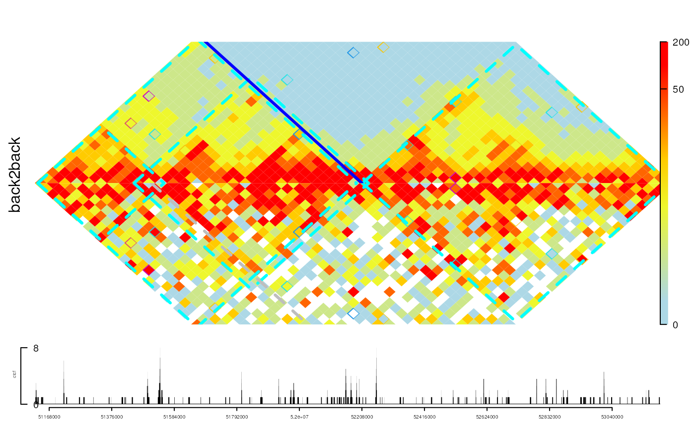
## view the interaction data back to back.
## Please make sure the data are normalized.
gi2 <- gi
set.seed(123)
gi2$score <- gi$score + rnorm(length(gi), sd = sd(gi$score))
back2back <- gi2track(gi, gi2)
## change the color
setTrackStyleParam(back2back, "breaks",
                   c(seq(from=0, to=50, by=10), 200))
setTrackStyleParam(back2back, "color",
                   c("lightblue", "yellow", "red"))
## chang the lim of y-axis (by default, [0, 1])
setTrackStyleParam(back2back, "ylim", c(0, .5))
viewTracks(trackList(ctcf, back2back, heightDist=c(1, 5)),
           gr=range, autoOptimizeStyle = TRUE)
addInteractionAnnotation(tads, "back2back", grid.lines,
                         gp=gpar(col="cyan", lwd=3, lty=2))
addInteractionAnnotation(-52208000, "back2back", gp=gpar(col="blue", lwd=3),
                         panel="top")
addInteractionAnnotation(51508000, "back2back", gp=gpar(col="gray", lwd=3, lty=2),
                         panel="bottom")
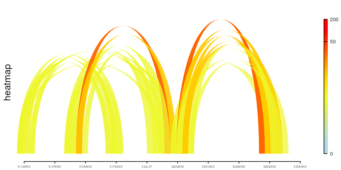
Plot chromatin interactions track as links.
setTrackStyleParam(heatmap, "tracktype", "link")
setTrackStyleParam(heatmap, "breaks",
                   c(seq(from=0, to=50, by=10), 200))
setTrackStyleParam(heatmap, "color",
                   c("lightblue", "yellow", "red"))
## filter the links to simulate the real data
keep <- distance(heatmap$dat, heatmap$dat2) > 5e5 & heatmap$dat$score>20
heatmap$dat <- heatmap$dat[keep]
heatmap$dat2 <- heatmap$dat2[keep]
viewTracks(trackList(heatmap), gr=range, autoOptimizeStyle = TRUE)
To import interactions data from “.hic” (reference to the script of
hic-straw and the documentation).
The function importGInteractions (trackViewer
version>=1.27.6) can be used to import data from .hic
format file.
hic <- system.file("extdata", "test_chr22.hic", package = "trackViewer",
                    mustWork=TRUE)
if(.Platform$OS.type!="windows"){
importGInteractions(file=hic, format="hic",
                    ranges=GRanges("22", IRanges(50000000, 100000000)),
                    out = "GInteractions")
}
## GInteractions object with 70 interactions and 1 metadata column:
## seqnames1 ranges1 seqnames2 ranges2 | score
## <Rle> <IRanges> <Rle> <IRanges> | <numeric>
## [1] 22 50000001-50100000 --- 22 50000001-50100000 | 26
## [2] 22 50000001-50100000 --- 22 50100001-50200000 | 2
## [3] 22 50100001-50200000 --- 22 50100001-50200000 | 22
## [4] 22 50100001-50200000 --- 22 50200001-50300000 | 7
## [5] 22 50200001-50300000 --- 22 50200001-50300000 | 31
## ... ... ... ... ... ... . ...
## [66] 22 50400001-50500000 --- 22 51200001-51300000 | 1
## [67] 22 50500001-50600000 --- 22 51200001-51300000 | 2
## [68] 22 50800001-50900000 --- 22 51200001-51300000 | 2
## [69] 22 51100001-51200000 --- 22 51200001-51300000 | 3
## [70] 22 51200001-51300000 --- 22 51200001-51300000 | 5
## -------
## regions: 13 ranges and 0 metadata columns
## seqinfo: 1 sequence from an unspecified genome; no seqlengthsAnother widely used genomic interaction data format is
.cool files and the cooler index contains
analyzed HiC data for hg19 and mm9 from many different sources. Those
files can be used as data resources for visualizations and annotations
(see ChIPpeakAnno::findEnhancers).
The importGInteractions function can also be used to import
data from .cool format (trackViewer
version>=1.27.6).
cool <- system.file("extdata", "test.mcool", package = "trackViewer",
                     mustWork=TRUE)
importGInteractions(file=cool, format="cool",
                    resolution = 2,
                    ranges=GRanges("chr1", IRanges(10, 28)),
                    out = "GInteractions")
Session Info
R version 4.4.1 (2024-06-14) Platform: x86_64-pc-linux-gnu Running under: Ubuntu 22.04.4 LTS
Matrix products: default BLAS: /usr/lib/x86_64-linux-gnu/openblas-pthread/libblas.so.3 LAPACK: /usr/lib/x86_64-linux-gnu/openblas-pthread/libopenblasp-r0.3.20.so; LAPACK version 3.10.0
locale: [1] LC_CTYPE=en_US.UTF-8 LC_NUMERIC=C
[3] LC_TIME=en_US.UTF-8 LC_COLLATE=en_US.UTF-8
[5] LC_MONETARY=en_US.UTF-8 LC_MESSAGES=en_US.UTF-8
[7] LC_PAPER=en_US.UTF-8 LC_NAME=C
[9] LC_ADDRESS=C LC_TELEPHONE=C
[11] LC_MEASUREMENT=en_US.UTF-8 LC_IDENTIFICATION=C
time zone: Etc/UTC tzcode source: system (glibc)
attached base packages: [1] grid stats4 stats graphics grDevices utils datasets [8] methods base
other attached packages: [1] InteractionSet_1.33.0
[2] SummarizedExperiment_1.35.1
[3] MatrixGenerics_1.17.0
[4] matrixStats_1.4.0
[5] org.Hs.eg.db_3.19.1
[6] TxDb.Hsapiens.UCSC.hg19.knownGene_3.2.2 [7]
GenomicFeatures_1.57.0
[8] AnnotationDbi_1.67.0
[9] Biobase_2.65.1
[10] trackViewer_1.41.6
[11] GenomicRanges_1.57.1
[12] GenomeInfoDb_1.41.1
[13] IRanges_2.39.2
[14] S4Vectors_0.43.2
[15] BiocGenerics_0.51.1
loaded via a namespace (and not attached): [1] strawr_0.0.92
RColorBrewer_1.1-3 rstudioapi_0.16.0
[4] jsonlite_1.8.8 magrittr_2.0.3 rmarkdown_2.28
[7] fs_1.6.4 BiocIO_1.15.2 zlibbioc_1.51.1
[10] ragg_1.3.2 vctrs_0.6.5 memoise_2.0.1
[13] Rsamtools_2.21.1 RCurl_1.98-1.16 base64enc_0.1-3
[16] htmltools_0.5.8.1 S4Arrays_1.5.7 progress_1.2.3
[19] curl_5.2.2 Rhdf5lib_1.27.0 rhdf5_2.49.0
[22] SparseArray_1.5.31 Formula_1.2-5 sass_0.4.9
[25] bslib_0.8.0 htmlwidgets_1.6.4 desc_1.4.3
[28] Gviz_1.49.0 httr2_1.0.3 cachem_1.1.0
[31] GenomicAlignments_1.41.0 lifecycle_1.0.4 pkgconfig_2.0.3
[34] Matrix_1.7-0 R6_2.5.1 fastmap_1.2.0
[37] GenomeInfoDbData_1.2.12 digest_0.6.37 colorspace_2.1-1
[40] textshaping_0.4.0 Hmisc_5.1-3 RSQLite_2.3.7
[43] filelock_1.0.3 fansi_1.0.6 httr_1.4.7
[46] abind_1.4-5 compiler_4.4.1 bit64_4.0.5
[49] htmlTable_2.4.3 backports_1.5.0 BiocParallel_1.39.0
[52] DBI_1.2.3 highr_0.11 biomaRt_2.61.3
[55] rappdirs_0.3.3 DelayedArray_0.31.11 rjson_0.2.22
[58] tools_4.4.1 foreign_0.8-87 nnet_7.3-19
[61] glue_1.7.0 restfulr_0.0.15 rhdf5filters_1.17.0
[64] checkmate_2.3.2 cluster_2.1.6 generics_0.1.3
[67] gtable_0.3.5 BSgenome_1.73.0 ensembldb_2.29.1
[70] data.table_1.16.0 hms_1.1.3 xml2_1.3.6
[73] utf8_1.2.4 XVector_0.45.0 pillar_1.9.0
[76] stringr_1.5.1 dplyr_1.1.4 BiocFileCache_2.13.0
[79] lattice_0.22-6 deldir_2.0-4 rtracklayer_1.65.0
[82] bit_4.0.5 biovizBase_1.53.0 tidyselect_1.2.1
[85] Biostrings_2.73.1 knitr_1.48 gridExtra_2.3
[88] ProtGenerics_1.37.1 xfun_0.47 stringi_1.8.4
[91] UCSC.utils_1.1.0 lazyeval_0.2.2 yaml_2.3.10
[94] evaluate_0.24.0 codetools_0.2-20 interp_1.1-6
[97] tibble_3.2.1 BiocManager_1.30.25 cli_3.6.3
[100] rpart_4.1.23 systemfonts_1.1.0 munsell_0.5.1
[103] jquerylib_0.1.4 Rcpp_1.0.13 dichromat_2.0-0.1
[106] grImport_0.9-7 dbplyr_2.5.0 png_0.1-8
[109] XML_3.99-0.17 parallel_4.4.1 pkgdown_2.1.0
[112] ggplot2_3.5.1 blob_1.2.4 prettyunits_1.2.0
[115] latticeExtra_0.6-30 jpeg_0.1-10 AnnotationFilter_1.29.0 [118]
bitops_1.0-8 txdbmaker_1.1.1 VariantAnnotation_1.51.0 [121] scales_1.3.0
crayon_1.5.3 BiocStyle_2.33.1
[124] rlang_1.1.4 KEGGREST_1.45.1