trackViewer Vignette: overview
Jianhong Ou, Lihua Julie Zhu
5 September 2024
trackViewer.RmdAbstract
Visualize mapped reads along with annotation as track layers for NGS dataset such as ChIP-seq, RNA-seq, miRNA-seq, DNA-seq, SNPs and methylation data.
Introduction
There are two packages available in Bioconductor for visualizing genomic data: rtracklayer and Gviz. rtracklayer provides an interface to genome browsers and associated annotation tracks. Gviz can be used to plot coverage and annotation tracks. TrackViewer is a lightweight visualization tool for generating interactive figures for publication. Not only can trackViewer be used to visualize coverage and annotation tracks, but it can also be employed to generate lollipop/dandelion plots that depict dense methylation/mutation/variant data to facilitate an integrative analysis of these multi-omics data. It leverages Gviz and rtracklayer, is easy to use, and has a low memory and cpu consumption. In addition, we implemented a web application of trackViewer leveraging Shiny package. The web application of trackViewer is available at https://github.com/jianhong/trackViewer.documentation/tree/master/trackViewerShinyApp.
Plot high dense methylation/mutation/variant data by dandelion plot
Plot genomic interaction data (HiC, cooler, etc) by viewTracks
library(Gviz)
library(rtracklayer)
library(trackViewer)
extdata <- system.file("extdata", package="trackViewer",
                       mustWork=TRUE)
gr <- GRanges("chr11", IRanges(122929275, 122930122), strand="-")
fox2 <- importScore(file.path(extdata, "fox2.bed"), format="BED",
                    ranges=gr)
fox2$dat <- coverageGR(fox2$dat)

viewTracks(trackList(fox2), gr=gr, autoOptimizeStyle=TRUE, newpage=FALSE)

dt <- DataTrack(range=fox2$dat[strand(fox2$dat)=="-"] ,
                genome="hg19", type="hist", name="fox2",
                window=-1, chromosome="chr11",
                fill.histogram="black", col.histogram="NA",
                background.title="white",
                col.frame="white", col.axis="black",
                col="black", col.title="black")
plotTracks(dt, from=122929275, to=122930122, strand="-")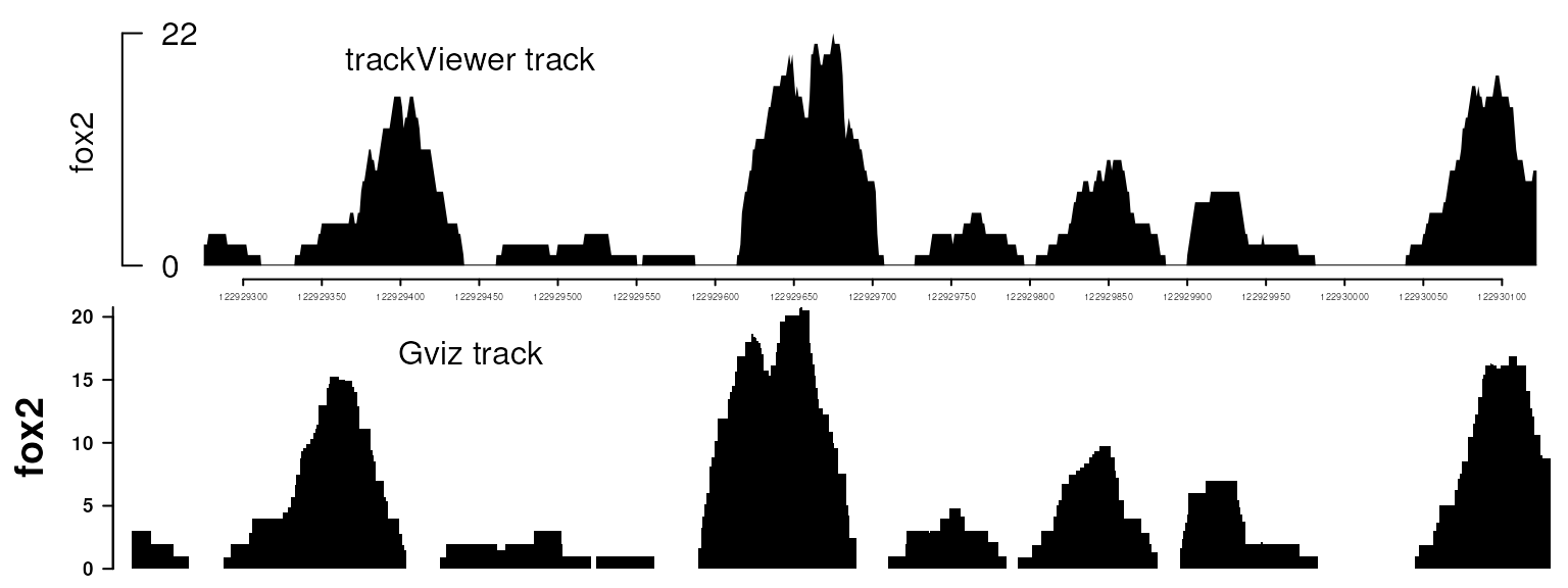
Plot data with Gviz and trackViewer. Please note that trackViewer can generate similar figure as Gviz with several lines of simple codes.
trackViewer not only has the functionalities to produce the figures generated by Gviz, as shown in the Figure above, but also provides additional plotting styles as shown in the Figure below. The mimimalist design requires minimum input from the users while retaining the flexibility to change the output style easily.
gr <- GRanges("chr1", IRanges(c(1, 6, 10), c(3, 6, 12)), score=c(3, 4, 1))
dt <- DataTrack(range=gr, data="score", type="hist")
plotTracks(dt, from=2, to=11)
tr <- new("track", dat=gr, type="data", format="BED")
viewTracks(trackList(tr), chromosome="chr1", start=2, end=11)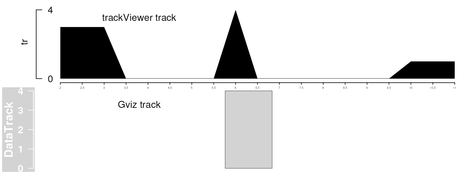
Plot data with Gviz and trackViewer. Note that trackViewer is not only including more details but also showing all the data involved in the given range.
Gviz requires huge memory space to handle big wig files. To solve this problem, we rewrote the import function in trackViewer by importing the entire file first and parsing it later when plot. As a result, trackViewer decreases the import time from 180 min to 21 min and the memory cost from 10G to 5.32G for a half giga wig file (GSM917672).
Browse
Steps of using trackViewer
Step 1. Import data
The function importScore is used to import BED, WIG, bedGraph or BigWig files. The function importBam is employed to import the bam files. Here is an example.
library(trackViewer)
extdata <- system.file("extdata", package="trackViewer",
                       mustWork=TRUE)
repA <- importScore(file.path(extdata, "cpsf160.repA_-.wig"),
                    file.path(extdata, "cpsf160.repA_+.wig"),
                    format="WIG")
## Because the wig file does not contain any strand info,
## we need to set it manually.
strand(repA$dat) <- "-"
strand(repA$dat2) <- "+"
The function coverageGR could be used to calculate the coverage after the data is imported.
fox2 <- importScore(file.path(extdata, "fox2.bed"), format="BED",
                    ranges=GRanges("chr11", IRanges(122830799, 123116707)))
dat <- coverageGR(fox2$dat)
## We can split the data by strand into two different track channels
## Here, we set the dat2 slot to save the negative strand info.

fox2$dat <- dat[strand(dat)=="+"]
fox2$dat2 <- dat[strand(dat)=="-"]
Step 2. Build the gene model
The gene model can be built for a given genomic range using geneModelFromTxdb function which uses the TranscriptDb object as the input.
library(TxDb.Hsapiens.UCSC.hg19.knownGene)
library(org.Hs.eg.db)
gr <- GRanges("chr11", IRanges(122929275, 122930122), strand="-")
trs <- geneModelFromTxdb(TxDb.Hsapiens.UCSC.hg19.knownGene,
                         org.Hs.eg.db,
                         gr=gr)
Users can generate a track object with the geneTrack function by inputting a TxDb and a list of gene Entrez IDs. Entrez IDs can be obtained from other types of gene IDs such as gene symbol by using the ID mapping function. For example, to generate a track object given gene FMR1 and human TxDb, refer to the code below.
Step 3. View the tracks
Use viewTracks function to plot data and annotation information along genomic coordinates. addGuideLine or addArrowMark can be used to highlight a specific region.
viewerStyle <- trackViewerStyle()
setTrackViewerStyleParam(viewerStyle, "margin", c(.1, .05, .02, .02))
trackList <- trackList(repA, fox2, trs)
vp <- viewTracks(trackList,
                 gr=gr, viewerStyle=viewerStyle,
                 autoOptimizeStyle=TRUE)
addGuideLine(c(122929767, 122929969), vp=vp)
addArrowMark(list(x=122929650,
                  y=2), # 2 means track 2 from the bottom.
             label="label",
             col="blue",
             vp=vp)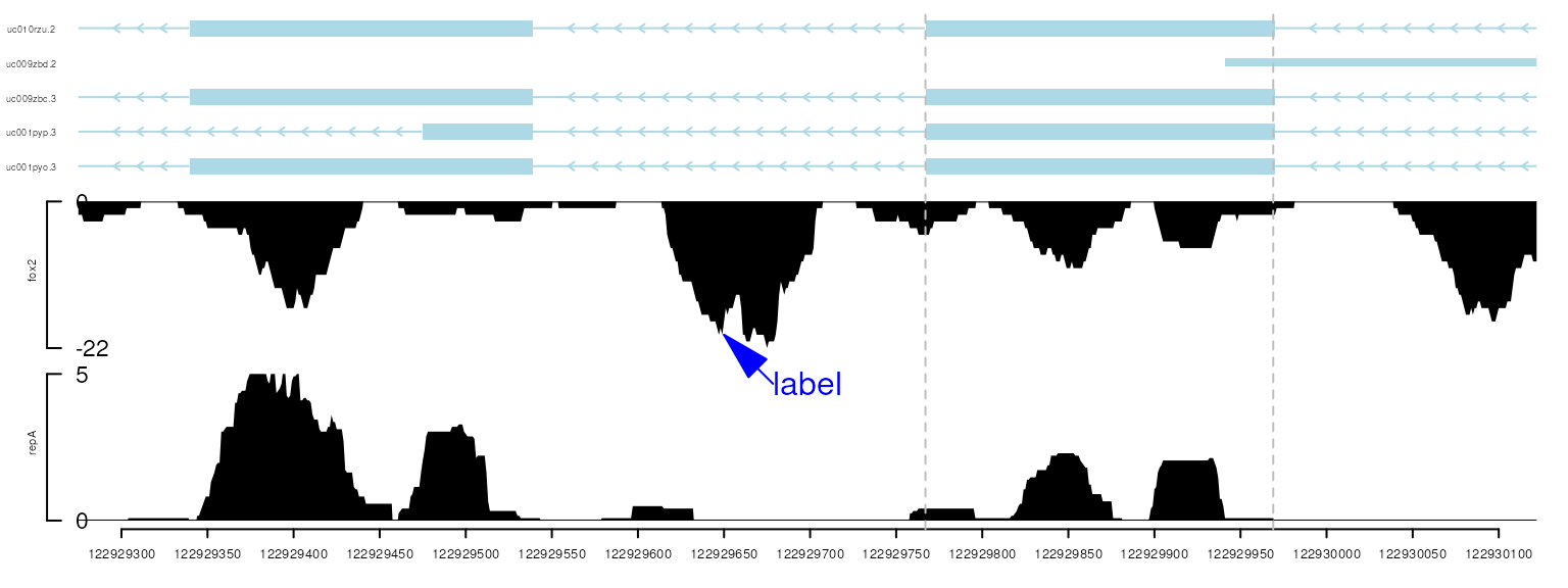
plot data and annotation information along genomic coordinates
For more details, please refer vignette changeTracksStyles.
Generate and edit an interactive plot using the browseTracks function
As shown above, figures produced by trackViewer are highly customizable, allowing users to alter the label, symbol, color, and size with various functions.
For users who prefer to modify the look and feel of a figure
interactively, they can use the function browseTracks to
draw interactive tracks, leveraging the htmlwidgets package.
browseTracks(trackList, gr=gr)interactive tracks
The videos at https://youtu.be/lSmeTu4WMlc and https://youtu.be/lvF0tnJiHQI illustrate how to generate
and modify an interactive plot. Please note that the interactive feature
is only fully implemented in version 1.19.14 or later.
Plot multiple genes in one track
library(TxDb.Hsapiens.UCSC.hg19.knownGene)
library(org.Hs.eg.db)
grW <- parse2GRanges("chr11:122,830,799-123,116,707")
ids <- getGeneIDsFromTxDb(grW, TxDb.Hsapiens.UCSC.hg19.knownGene)
symbols <- mget(ids, org.Hs.egSYMBOL)
genes <- geneTrack(ids, TxDb.Hsapiens.UCSC.hg19.knownGene,
                   symbols, asList=FALSE)
# set color to the gene
genes$dat$color <- as.numeric(factor(genes$dat$featureID))
optSty <- optimizeStyle(trackList(repA, fox2, genes), theme="safe")
trackListW <- optSty$tracks
viewerStyleW <- optSty$style
viewTracks(trackListW, gr=grW, viewerStyle=viewerStyleW)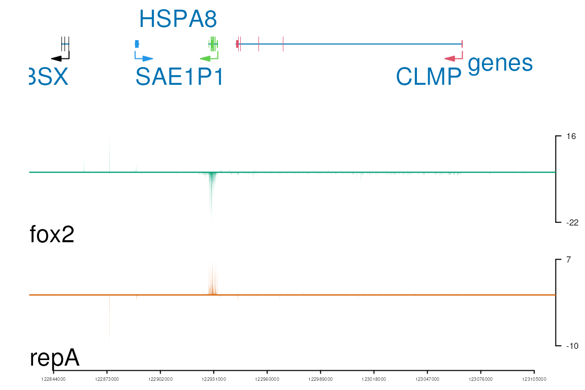
Plot multiple genes in one track
Operators
If you are interested in drawing a combined track from two input tracks, e.g, adding or substractiong one from the other, then you can try one of the operators such as + and - as showing below.
newtrack <- repA
## Must keep the same format for dat and dat2
newtrack <- parseWIG(newtrack, "chr11", 122929275, 122930122)
newtrack$dat2 <- newtrack$dat
newtrack$dat <- fox2$dat2
setTrackStyleParam(newtrack, "color", c("#4A95E0", "#CF5D6D"))
viewTracks(trackList(newtrack, trs),
           gr=gr, viewerStyle=viewerStyle, operator="+")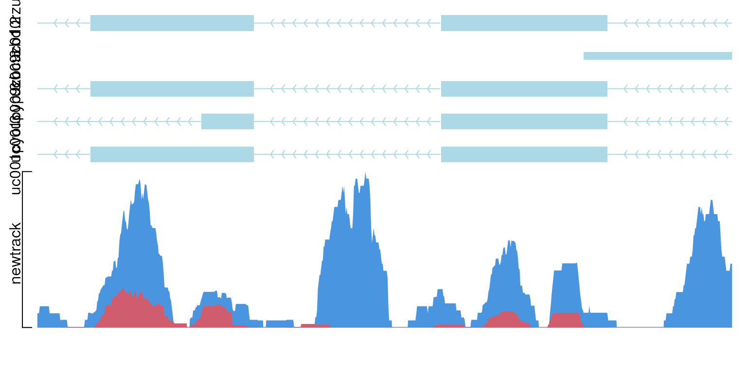
show data with operator “+”
viewTracks(trackList(newtrack, trs), gr=gr, viewerStyle=viewerStyle, operator="-")
show data with operator “-”
Multiple operators are acceptable.
viewTracks(trackList(newtrack, newtrack, newtrack, trs), gr=gr, viewerStyle=viewerStyle, operator=c(NA, "-", "+"))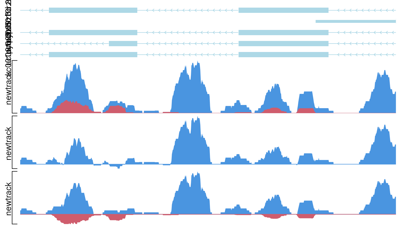
show data with multiple operators
Alternatively, you can try GRoperator before viewing tracks.
newtrack$dat <- GRoperator(newtrack$dat, newtrack$dat2, col="score", operator="-")
newtrack$dat2 <- GRanges()
viewTracks(trackList(newtrack, trs), gr=gr, viewerStyle=viewerStyle)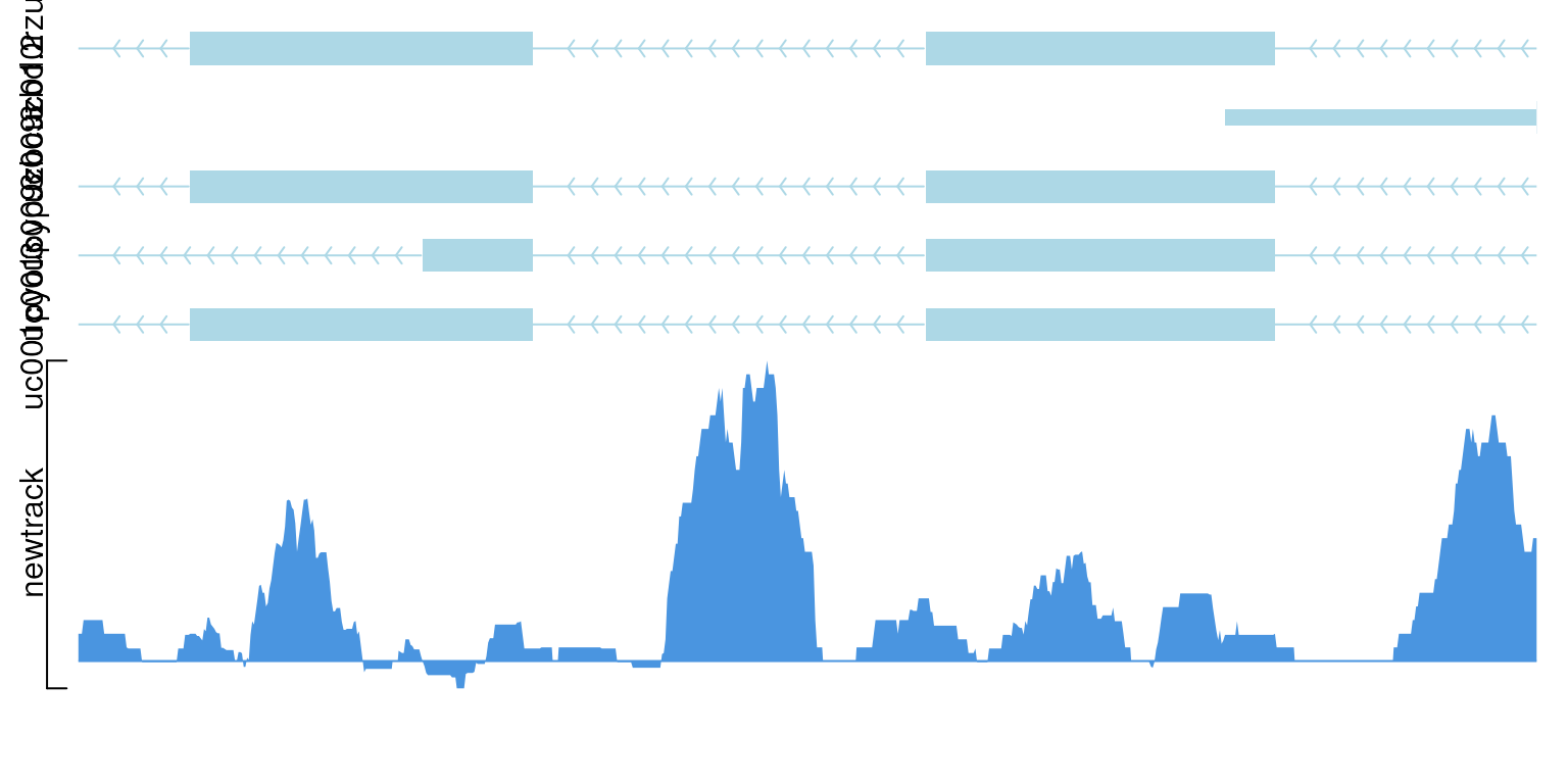
show data with operator “-”
Lolliplot
The lolliplot function is for the visualization of the
methylation/variant/mutation data. For more details, please refer vignette lollipopPlot.
library(trackViewer)
features <- GRanges("chr1", IRanges(c(1, 501, 1001),
                                    width=c(120, 400, 405),
                                    names=paste0("block", 1:3)),
                    fill = c("#FF8833", "#51C6E6", "#DFA32D"),
                    height = c(0.02, 0.05, 0.08))
SNP <- c(10, 100, 105, 108, 400, 410, 420, 600, 700, 805, 840, 1400, 1402)
sample.gr <- GRanges("chr1", IRanges(SNP, width=1, names=paste0("snp", SNP)),
                     color = sample.int(6, length(SNP), replace=TRUE),
                     score = sample.int(5, length(SNP), replace = TRUE))
lolliplot(sample.gr, features)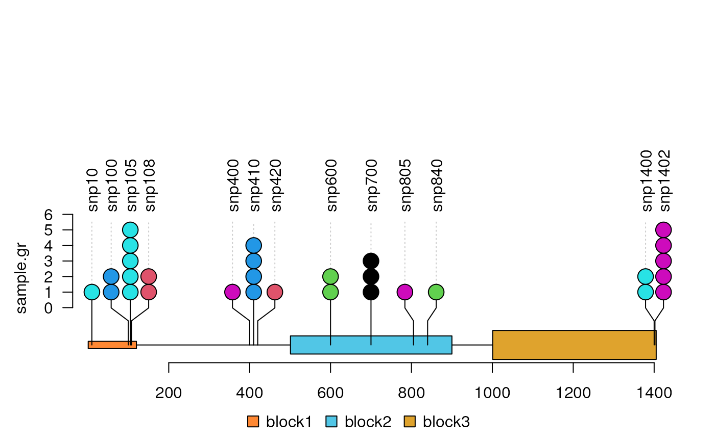
Dandelion Plot
Dandelion Plot is used to plot high dense of mutation/methylation data. For more details, please refer vignette dandelionPlot.
library(trackViewer)
library(TxDb.Hsapiens.UCSC.hg19.knownGene)
library(org.Hs.eg.db)
methy <- import(system.file("extdata", "methy.bed", package="trackViewer"), "BED")
gr <- GRanges("chr22", IRanges(50968014, 50970514, names="TYMP"))
trs <- geneModelFromTxdb(TxDb.Hsapiens.UCSC.hg19.knownGene,
                         org.Hs.eg.db,
                         gr=gr)
features <- c(range(trs[[1]]$dat), range(trs[[5]]$dat))
names(features) <- c(trs[[1]]$name, trs[[5]]$name)
features$fill <- c("lightblue", "mistyrose")
features$height <- c(.02, .04)
dandelion.plot(methy, features, ranges=gr, type="pin")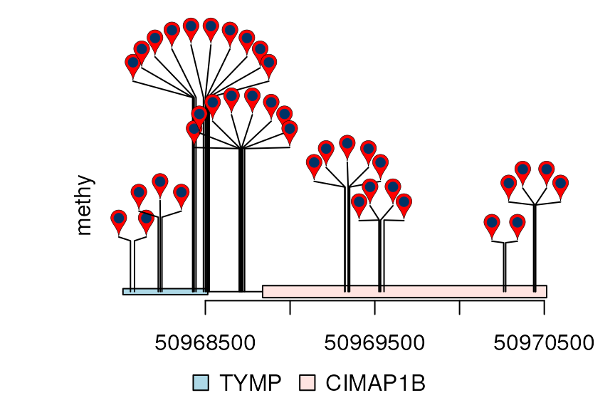
Plot chromatin interactions data
Plot chromatin interactions heatmap as tracks. For more details, please refer vignette plotInteractionData.
library(InteractionSet)
gi <- readRDS(system.file("extdata", "nij.chr6.51120000.53200000.gi.rds", package="trackViewer"))
head(gi)
## GInteractions object with 6 interactions and 1 metadata column:
## seqnames1 ranges1 seqnames2 ranges2 | score
## <Rle> <IRanges> <Rle> <IRanges> | <numeric>
## [1] chr6 51120000-51160000 --- chr6 51120000-51160000 | 45.1227
## [2] chr6 51120000-51160000 --- chr6 51160000-51200000 | 35.0006
## [3] chr6 51120000-51160000 --- chr6 51200000-51240000 | 44.7322
## [4] chr6 51120000-51160000 --- chr6 51240000-51280000 | 29.3507
## [5] chr6 51120000-51160000 --- chr6 51280000-51320000 | 38.8417
## [6] chr6 51120000-51160000 --- chr6 51320000-51360000 | 31.7063
## -------
## regions: 53 ranges and 0 metadata columns
## seqinfo: 1 sequence from an unspecified genome; no seqlengths
range <- GRanges("chr6", IRanges(51120000, 53200000))
tr <- gi2track(gi)
ctcf <- readRDS(system.file("extdata", "ctcf.sample.rds",
                            package="trackViewer"))
## change the color
setTrackStyleParam(tr, "breaks",
                   c(seq(from=0, to=50, by=10), 200))
setTrackStyleParam(tr, "color",
                   c("lightblue", "yellow", "red"))
viewTracks(trackList(ctcf, tr, heightDist=c(1, 3)), gr=range,
           autoOptimizeStyle = TRUE)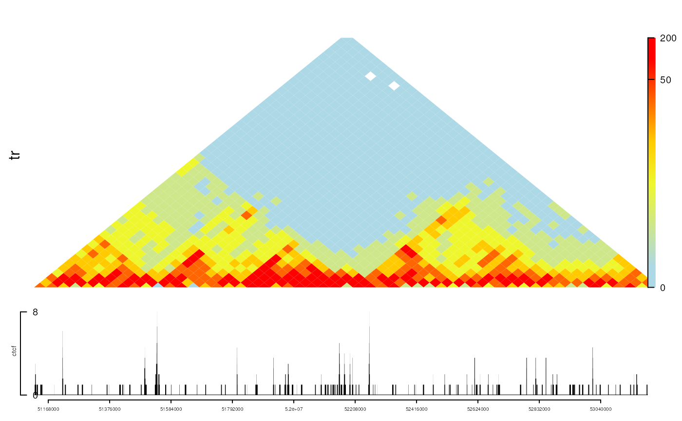
Ideogram Plot
Plot ideograms with a list of chromosomes and a genome.
ideo <- loadIdeogram("hg38", chrom=c("chr1", "chr3", "chr4", 'chr21', "chr22"))
dataList <- trim(ideo)
dataList$score <- as.numeric(as.factor(dataList$gieStain))
dataList <- dataList[dataList$gieStain!="gneg"]
dataList <- GRangesList(dataList)
ideogramPlot(ideo, dataList,
            layout=list("chr1", c("chr3", "chr22"),
                        c("chr4", "chr21")))
Web application of trackViewer
We created a web application of trackViewer (available in 1.19.14 or later) by leveraging the R package Shiny. The web application of trackViewer and sample data are available at https://github.com/jianhong/trackViewer.documentation/tree/master/trackViewerShinyApp. Here is a demo on how to to use the web application at https://www.nature.com/articles/s41592-019-0430-y#Sec2 Supplementary Video 5.
Session Info
R version 4.4.1 (2024-06-14) Platform: x86_64-pc-linux-gnu Running under: Ubuntu 22.04.4 LTS
Matrix products: default BLAS: /usr/lib/x86_64-linux-gnu/openblas-pthread/libblas.so.3 LAPACK: /usr/lib/x86_64-linux-gnu/openblas-pthread/libopenblasp-r0.3.20.so; LAPACK version 3.10.0
locale: [1] LC_CTYPE=en_US.UTF-8 LC_NUMERIC=C
[3] LC_TIME=en_US.UTF-8 LC_COLLATE=en_US.UTF-8
[5] LC_MONETARY=en_US.UTF-8 LC_MESSAGES=en_US.UTF-8
[7] LC_PAPER=en_US.UTF-8 LC_NAME=C
[9] LC_ADDRESS=C LC_TELEPHONE=C
[11] LC_MEASUREMENT=en_US.UTF-8 LC_IDENTIFICATION=C
time zone: Etc/UTC tzcode source: system (glibc)
attached base packages: [1] grid stats4 stats graphics grDevices utils datasets [8] methods base
other attached packages: [1] InteractionSet_1.33.0
[2] httr_1.4.7
[3] VariantAnnotation_1.51.0
[4] Rsamtools_2.21.1
[5] Biostrings_2.73.1
[6] XVector_0.45.0
[7] SummarizedExperiment_1.35.1
[8] MatrixGenerics_1.17.0
[9] matrixStats_1.4.0
[10] org.Hs.eg.db_3.19.1
[11] TxDb.Hsapiens.UCSC.hg19.knownGene_3.2.2 [12]
GenomicFeatures_1.57.0
[13] AnnotationDbi_1.67.0
[14] Biobase_2.65.1
[15] Gviz_1.49.0
[16] rtracklayer_1.65.0
[17] trackViewer_1.41.6
[18] GenomicRanges_1.57.1
[19] GenomeInfoDb_1.41.1
[20] IRanges_2.39.2
[21] S4Vectors_0.43.2
[22] BiocGenerics_0.51.1
loaded via a namespace (and not attached): [1] strawr_0.0.92
RColorBrewer_1.1-3 rstudioapi_0.16.0
[4] jsonlite_1.8.8 magrittr_2.0.3 rmarkdown_2.28
[7] fs_1.6.4 BiocIO_1.15.2 zlibbioc_1.51.1
[10] ragg_1.3.2 vctrs_0.6.5 memoise_2.0.1
[13] RCurl_1.98-1.16 base64enc_0.1-3 htmltools_0.5.8.1
[16] S4Arrays_1.5.7 progress_1.2.3 curl_5.2.2
[19] Rhdf5lib_1.27.0 rhdf5_2.49.0 SparseArray_1.5.31
[22] Formula_1.2-5 sass_0.4.9 bslib_0.8.0
[25] htmlwidgets_1.6.4 desc_1.4.3 httr2_1.0.3
[28] cachem_1.1.0 GenomicAlignments_1.41.0 lifecycle_1.0.4
[31] pkgconfig_2.0.3 Matrix_1.7-0 R6_2.5.1
[34] fastmap_1.2.0 GenomeInfoDbData_1.2.12 digest_0.6.37
[37] colorspace_2.1-1 textshaping_0.4.0 Hmisc_5.1-3
[40] RSQLite_2.3.7 filelock_1.0.3 fansi_1.0.6
[43] abind_1.4-5 compiler_4.4.1 bit64_4.0.5
[46] htmlTable_2.4.3 backports_1.5.0 BiocParallel_1.39.0
[49] DBI_1.2.3 highr_0.11 biomaRt_2.61.3
[52] rappdirs_0.3.3 DelayedArray_0.31.11 rjson_0.2.22
[55] tools_4.4.1 foreign_0.8-87 nnet_7.3-19
[58] glue_1.7.0 restfulr_0.0.15 rhdf5filters_1.17.0
[61] checkmate_2.3.2 cluster_2.1.6 generics_0.1.3
[64] gtable_0.3.5 BSgenome_1.73.0 ensembldb_2.29.1
[67] data.table_1.16.0 hms_1.1.3 xml2_1.3.6
[70] utf8_1.2.4 pillar_1.9.0 stringr_1.5.1
[73] dplyr_1.1.4 BiocFileCache_2.13.0 lattice_0.22-6
[76] deldir_2.0-4 bit_4.0.5 biovizBase_1.53.0
[79] tidyselect_1.2.1 knitr_1.48 gridExtra_2.3
[82] ProtGenerics_1.37.1 xfun_0.47 stringi_1.8.4
[85] UCSC.utils_1.1.0 lazyeval_0.2.2 yaml_2.3.10
[88] evaluate_0.24.0 codetools_0.2-20 interp_1.1-6
[91] tibble_3.2.1 BiocManager_1.30.25 cli_3.6.3
[94] rpart_4.1.23 systemfonts_1.1.0 munsell_0.5.1
[97] jquerylib_0.1.4 Rcpp_1.0.13 dichromat_2.0-0.1
[100] grImport_0.9-7 dbplyr_2.5.0 png_0.1-8
[103] XML_3.99-0.17 parallel_4.4.1 pkgdown_2.1.0
[106] ggplot2_3.5.1 blob_1.2.4 prettyunits_1.2.0
[109] latticeExtra_0.6-30 jpeg_0.1-10 AnnotationFilter_1.29.0 [112]
bitops_1.0-8 txdbmaker_1.1.1 scales_1.3.0
[115] crayon_1.5.3 BiocStyle_2.33.1 rlang_1.1.4
[118] KEGGREST_1.45.1