trackViewer Vignette: change the track styles

Abstract

Visualize mapped reads along with annotation as track layers for NGS dataset such as ChIP-seq, RNA-seq, miRNA-seq, DNA-seq, SNPs and methylation data.

Prepare toy data

First, we import the sample data.

library(trackViewer)
extdata <- system.file("extdata", package="trackViewer",
                       mustWork=TRUE)
repA <- importScore(file.path(extdata, "cpsf160.repA_-.wig"),
                    file.path(extdata, "cpsf160.repA_+.wig"),
                    format="WIG")
## Because the wig file does not contain any strand info, 
## we need to set it manually.
strand(repA$dat) <- "-"
strand(repA$dat2) <- "+"

fox2 <- importScore(file.path(extdata, "fox2.bed"), format="BED",
                    ranges=GRanges("chr11", IRanges(122830799, 123116707)))
dat <- coverageGR(fox2$dat)
## We can split the data by strand into two different track channels
## Here, we set the dat2 slot to save the negative strand info. 
 
fox2$dat <- dat[strand(dat)=="+"]
fox2$dat2 <- dat[strand(dat)=="-"]

library(TxDb.Hsapiens.UCSC.hg19.knownGene)
library(org.Hs.eg.db)
gr <- GRanges("chr11", IRanges(122929275, 122930122), strand="-")
trs <- geneModelFromTxdb(TxDb.Hsapiens.UCSC.hg19.knownGene,
                         org.Hs.eg.db,
                         gr=gr)

optSty <- optimizeStyle(trackList(repA, fox2, trs))
trackList <- optSty$tracks
viewerStyle <- optSty$style

Using the `browseTracks` function as a helper

Since version 1.33.6, the interactive plot generated by browseTracks function will print the psuedocode about how to change the track styles at the bottom, which can be used as a quick reference.

browseTracks(trackList, gr=gr)

Adjust the x-axis or the X scale

In most cases, researchers are interested in the relative position of the peaks in the gene. Sometimes, margin needs to be adjusted to be able to show the entire gene model. The Figure below shows how to add an X scale (x-scale) and remove the x-axis using the setTrackXscaleParam and setTrackViewerStyleParam functions.

setTrackViewerStyleParam(viewerStyle, "xaxis", FALSE)
setTrackViewerStyleParam(viewerStyle, "margin", c(.01, .05, .01, .01))
setTrackXscaleParam(trackList[[1]], "draw", TRUE)
setTrackXscaleParam(trackList[[1]], "gp", list(cex=0.8))
viewTracks(trackList, gr=gr, viewerStyle=viewerStyle)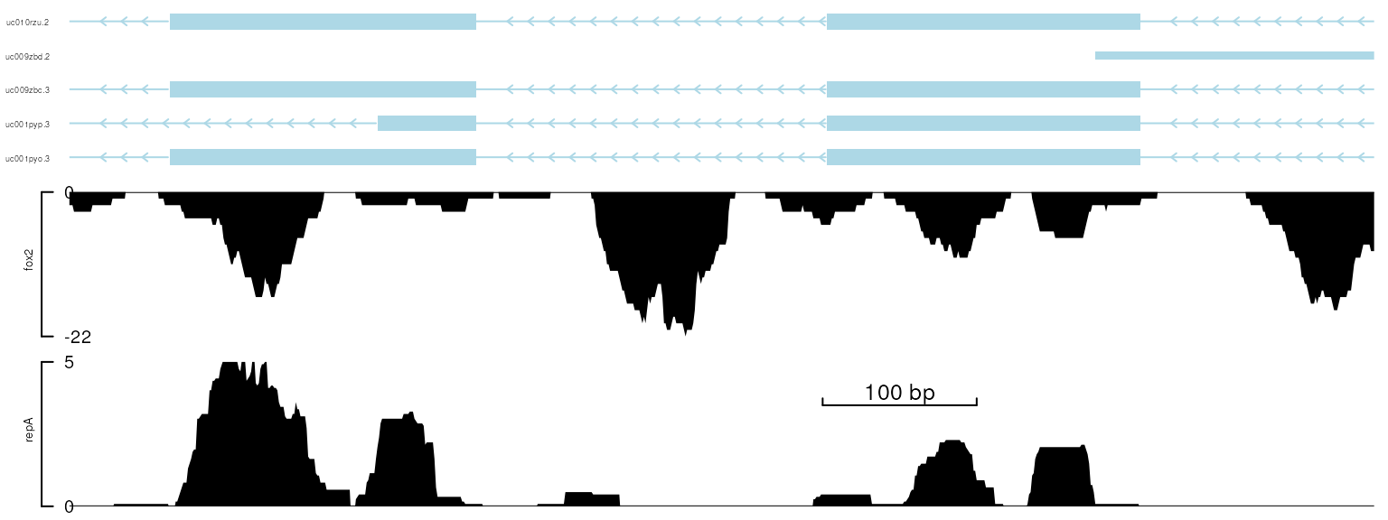

plot data with x-scale

setTrackXscaleParam(trackList[[1]], attr="position", 
                    value=list(x=122929700, y=3, label=200))
viewTracks(trackList, gr=gr, viewerStyle=viewerStyle)

plot data with x-scale

Adjust the y-axis

The y-axis can be put to the right side of the track by setting the main slot to FALSE in the y-axis slot of each track. In addition, the limit of y-axis (ylim) can be set by setTrackStyleParam.

setTrackViewerStyleParam(viewerStyle, "margin", c(.01, .05, .01, .05))
for(i in 1:2){
    setTrackYaxisParam(trackList[[i]], "main", FALSE)
}
## Adjust the limit of y-axis
setTrackStyleParam(trackList[[1]], "ylim", c(0, 25))
setTrackStyleParam(trackList[[2]], "ylim", c(-25, 0))
## The y-axis tick labels can be turn off/on by setting the 'label' to FALSE/TRUE
#setTrackYaxisParam(trackList[[1]], 'label', TRUE)
viewTracks(trackList, gr=gr, viewerStyle=viewerStyle)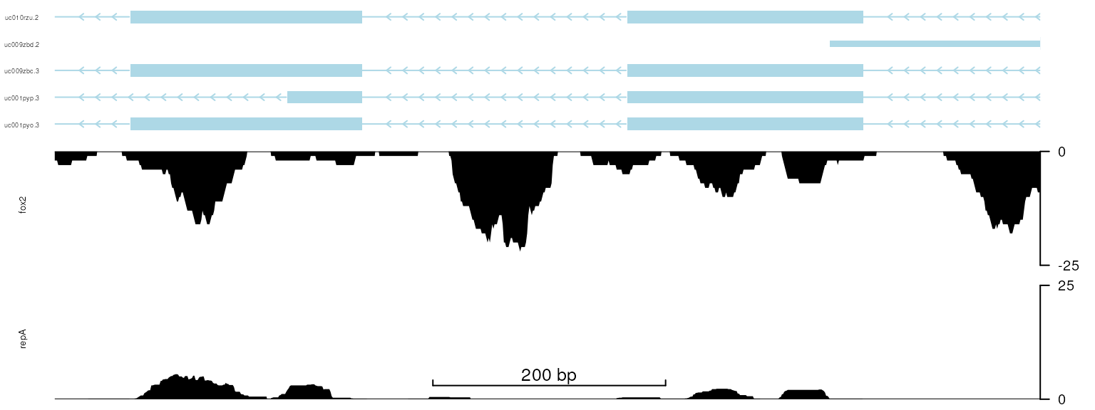

plot data with y-axis in right side

The function setTrackYaxisParam can be sued to adjust the track color/size/etc of y-axis and the y-axis labels.

## change the 
setTrackYaxisParam(trackList[[1]], "gp", list(cex=.8, col="green"))
setTrackYaxisParam(trackList[[2]], "gp", list(cex=.8, col="blue"))
viewTracks(trackList, gr=gr, viewerStyle=viewerStyle)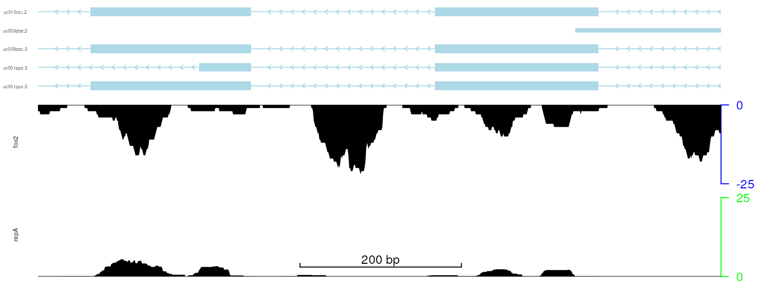

plot data with adjusted track color

Adjust the label of y-axis

The style of y-axis can be changed by setting the ylabgp slot in the style of each track.

setTrackStyleParam(trackList[[1]], "ylabgp", list(cex=.8, col="green"))
## set cex to avoid automatic adjust
setTrackStyleParam(trackList[[2]], "ylabgp", list(cex=.8, col="blue"))
setTrackStyleParam(trackList[[2]], "marginBottom", .2)
viewTracks(trackList, gr=gr, viewerStyle=viewerStyle)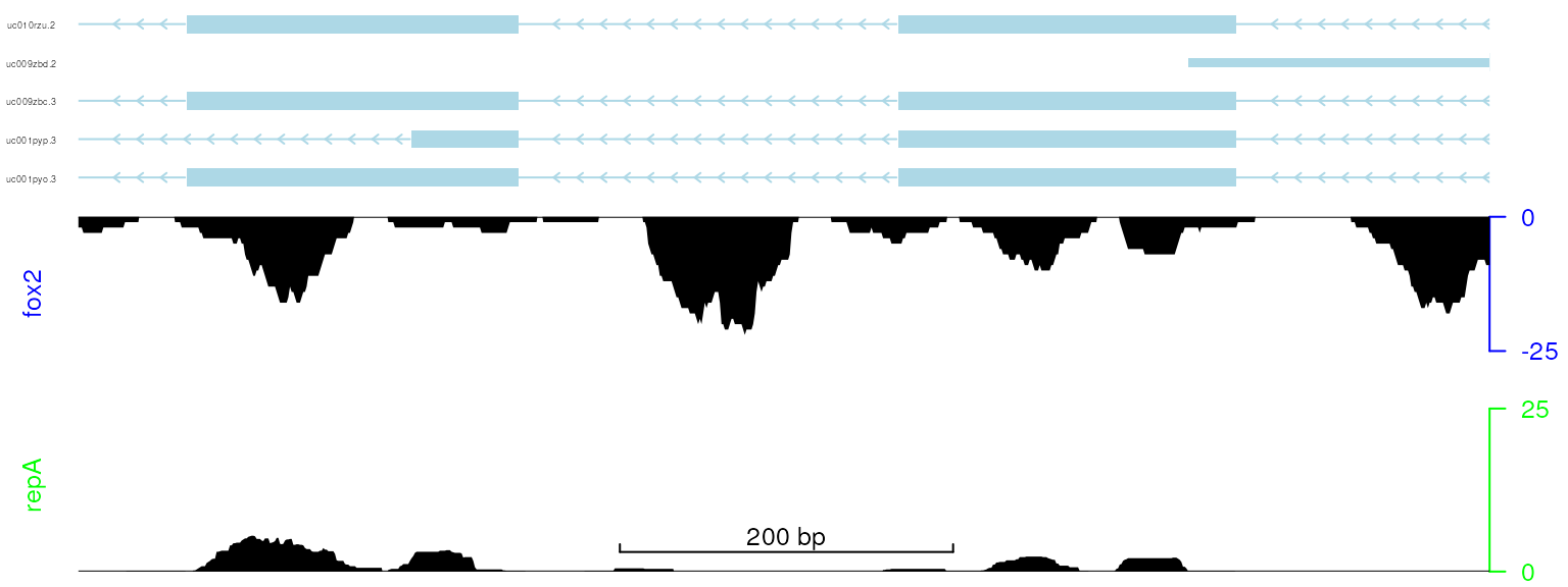

plot data with adjusted color and size of y-axis label

The y-axis label can be put at the top or the bottom of each track.

setTrackStyleParam(trackList[[1]], "ylabpos", "bottomleft")
setTrackStyleParam(trackList[[2]], "ylabpos", "topright")
setTrackStyleParam(trackList[[2]], "marginTop", .2)
viewTracks(trackList, gr=gr, viewerStyle=viewerStyle)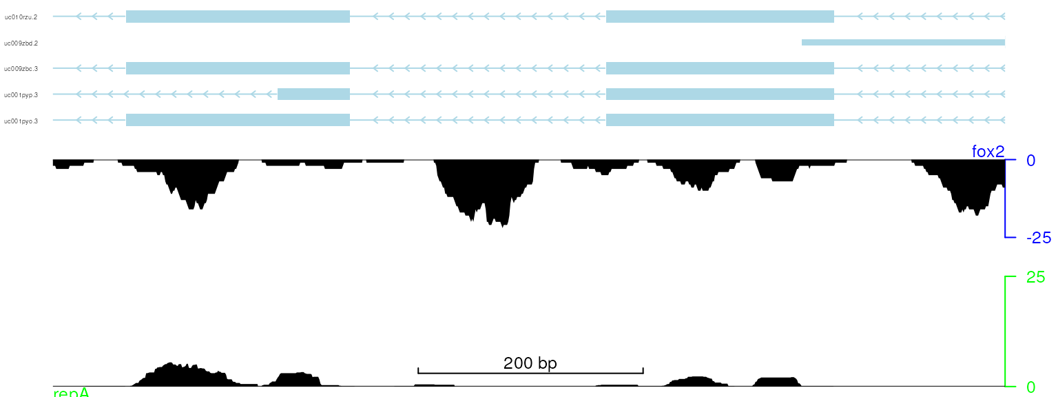

plot data with adjusted y-axis label position

For each transcript, the transcript name can be put on the upstream or downstream of the transcript.

trackListN <- trackList
setTrackStyleParam(trackListN[[3]], "ylabpos", "upstream")
setTrackStyleParam(trackListN[[4]], "ylabpos", "downstream")
## set cex to avoid automatic adjust
setTrackStyleParam(trackListN[[3]], "ylabgp", list(cex=.6))
setTrackStyleParam(trackListN[[4]], "ylabgp", list(cex=.6))
gr1 <- range(unname(unlist(GRangesList(sapply(trs, function(.ele) .ele$dat)))))
start(gr1) <- start(gr1) - 2000
end(gr1) <- end(gr1) + 2000
viewTracks(trackListN, gr=gr1, viewerStyle=viewerStyle)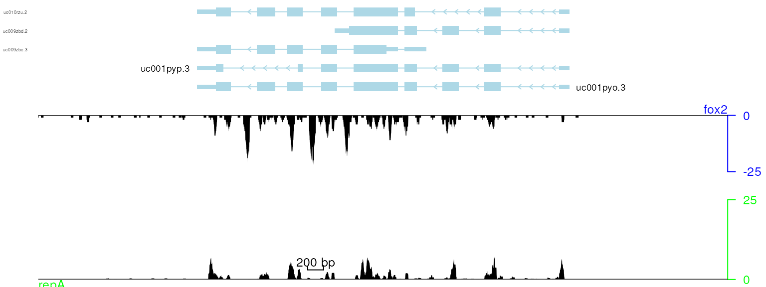

plot data with adjusted transcripts name position

Adjust the track color

The track color can be changed by setting the color slot in the style of each track. The first color is for the dat slot of track and the second color is for the dat2 slot.

setTrackStyleParam(trackList[[1]], "color", c("green", "black"))
setTrackStyleParam(trackList[[2]], "color", c("black", "blue"))
for(i in 3:length(trackList)) 
    setTrackStyleParam(trackList[[i]], "color", "black")
viewTracks(trackList, gr=gr, viewerStyle=viewerStyle)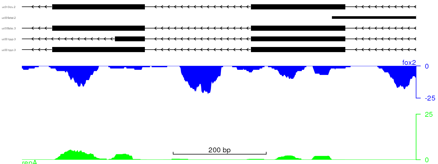

plot data with adjusted track color

Adjust the track height

The track height can be changed by setting the height slot in the style of each track. However, the total height for all the tracks should be 1.

trackListH <- trackList
setTrackStyleParam(trackListH[[1]], "height", .1)
setTrackStyleParam(trackListH[[2]], "height", .44)
for(i in 3:length(trackListH)){
    setTrackStyleParam(trackListH[[i]], "height", 
                       (1-(0.1+0.44))/(length(trackListH)-2))
}
viewTracks(trackListH, gr=gr, viewerStyle=viewerStyle)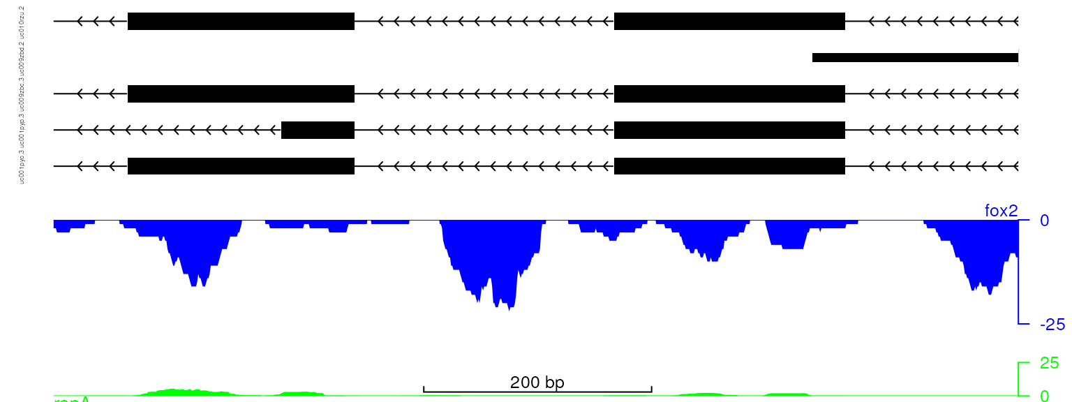

plot data with adjusted track height

Change the track names

The track names such as gene model names can be edited easily by changing the names of trackList.

names(trackList) <- c("cpsf160", "fox2", rep("HSPA8", 5))
viewTracks(trackList, gr=gr, viewerStyle=viewerStyle)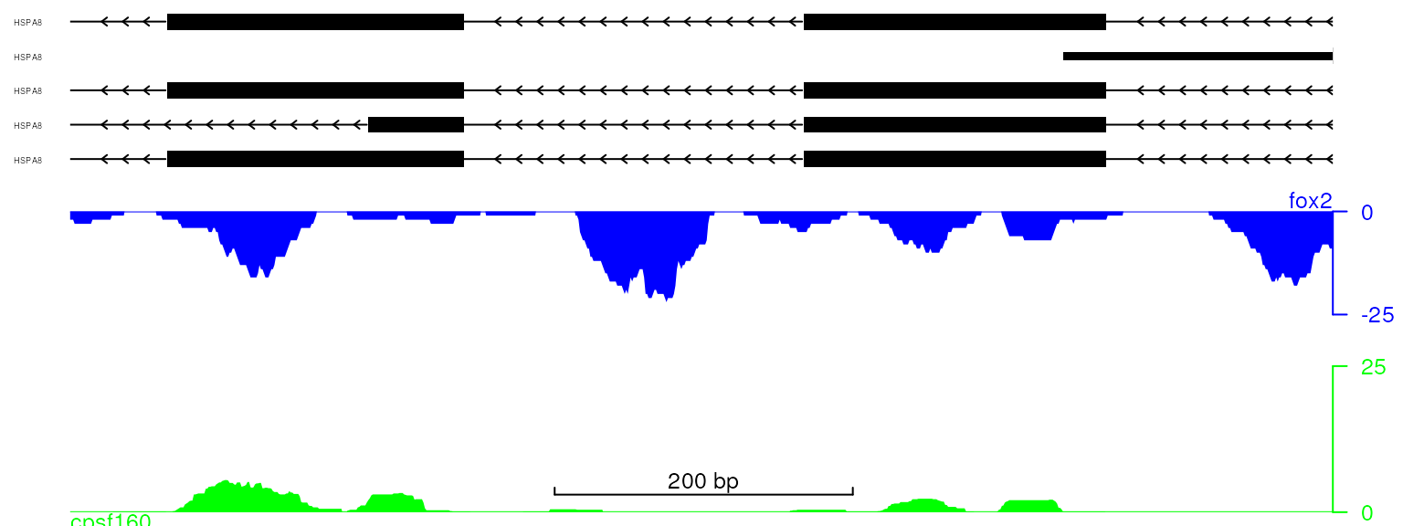

change the track names

Show paired data in the same track

trackViewer can be used to show to-be-compared data in the same track side by side.

cpsf160 <- importScore(file.path(extdata, "cpsf160.repA_-.wig"),
                       file.path(extdata, "cpsf160.repB_-.wig"),
                       format="WIG")
strand(cpsf160$dat) <- strand(cpsf160$dat2) <- "-"
setTrackStyleParam(cpsf160, "color", c("black", "red"))
viewTracks(trackList(trs, cpsf160), gr=gr, viewerStyle=viewerStyle)

show two data in the same track

Flip the x-axis

The x-axis can be horizotally flipped for the genes in the negative strand.

viewerStyleF <- viewerStyle
setTrackViewerStyleParam(viewerStyleF, "flip", TRUE)
setTrackViewerStyleParam(viewerStyleF, "xaxis", TRUE)
setTrackViewerStyleParam(viewerStyleF, "margin", c(.1, .05, .01, .01))
vp <- viewTracks(trackList, gr=gr, viewerStyle=viewerStyleF)
addGuideLine(c(122929767, 122929969), vp=vp)
addArrowMark(list(x=122929650,
                  y=2),
             label="label",
             col="blue",
             vp=vp)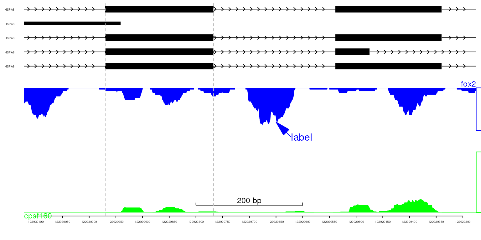

show data in the flipped track

Optimize the theme

Currently, we support two themes: bw (black and white) and col (colored).

optSty <- optimizeStyle(trackList(repA, fox2, trs), theme="bw")
trackList <- optSty$tracks
viewerStyle <- optSty$style
vp <- viewTracks(trackList, gr=gr, viewerStyle=viewerStyle)

balck & white theme

optSty <- optimizeStyle(trackList(repA, fox2, trs), theme="col")
trackList <- optSty$tracks
viewerStyle <- optSty$style
vp <- viewTracks(trackList, gr=gr, viewerStyle=viewerStyle)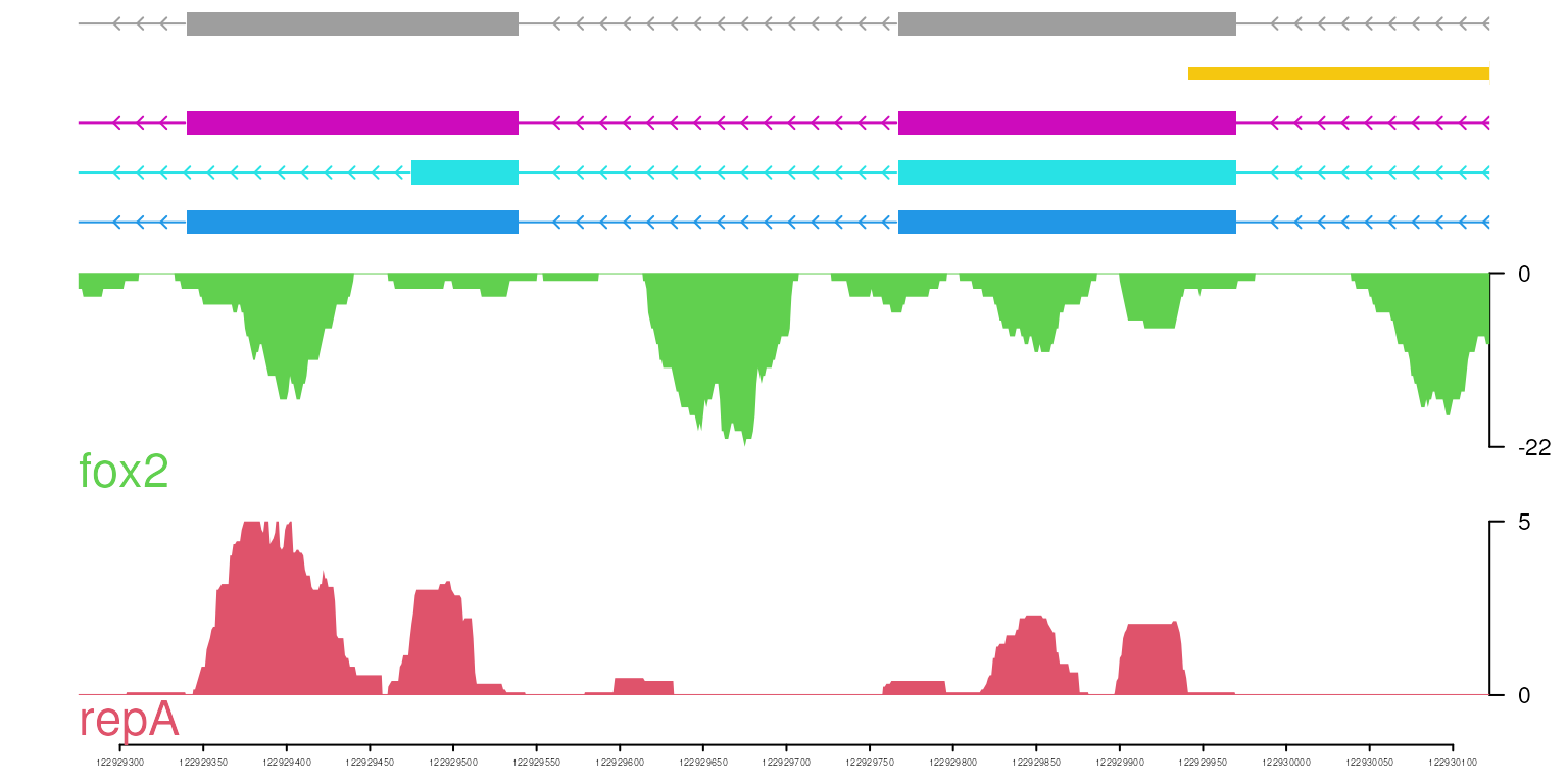

colorful theme

optSty <- optimizeStyle(trackList(repA, fox2, trs), theme="safe")
trackList <- optSty$tracks
viewerStyle <- optSty$style
vp <- viewTracks(trackList, gr=gr, viewerStyle=viewerStyle)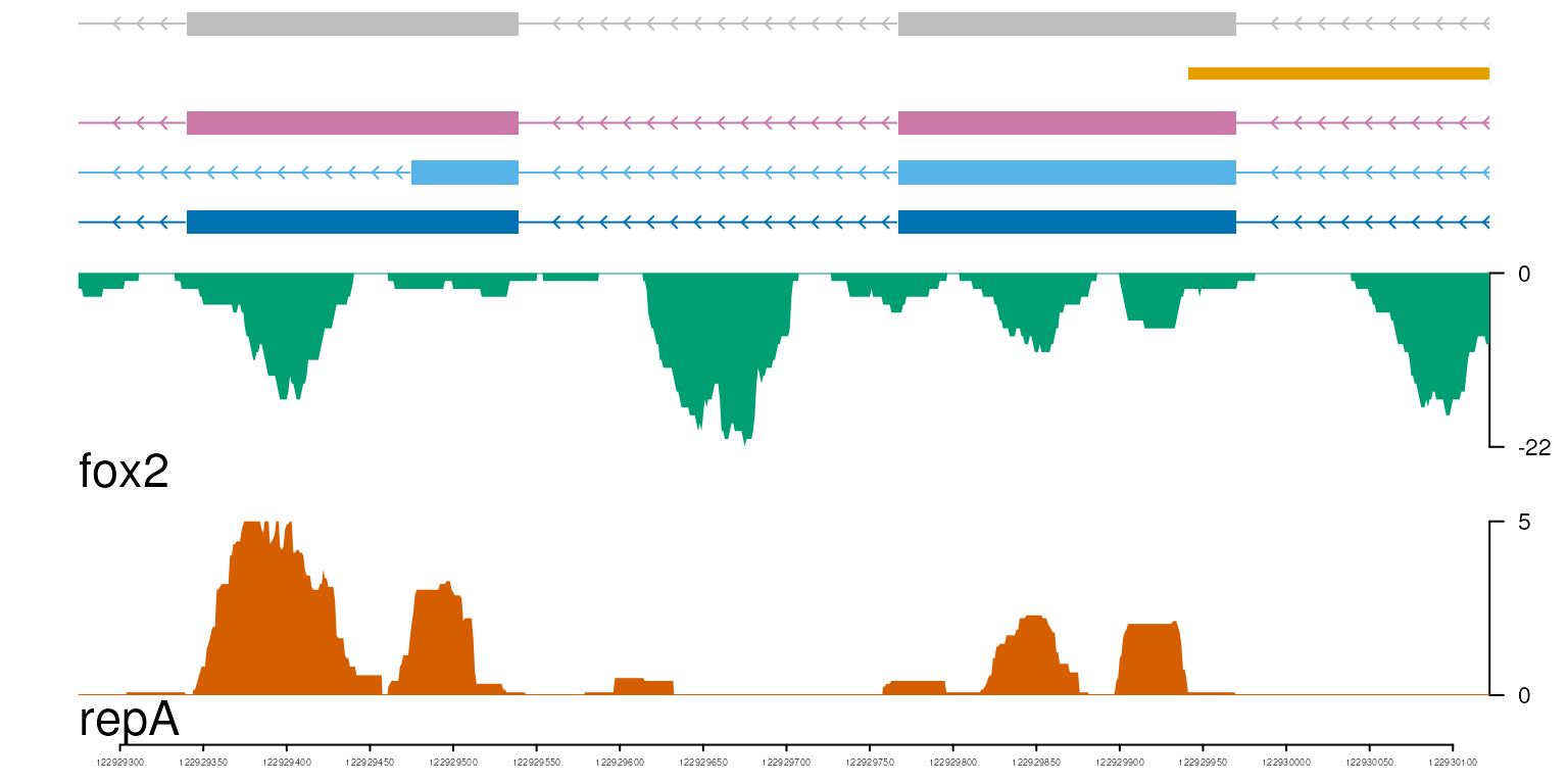

safe theme

Plot with breaks

We could plot the tracks with breaks by setting multiple genomic ranges.

gr.breaks <- GRanges("chr11", 
                     IRanges(c(122929275, 122929575, 122929775), 
                             c(122929555, 122929725, 122930122)), 
                     strand="-", percentage=c(.4, .2, .4))
vp <- viewTracks(trackList, gr=gr.breaks, viewerStyle=viewerStyle)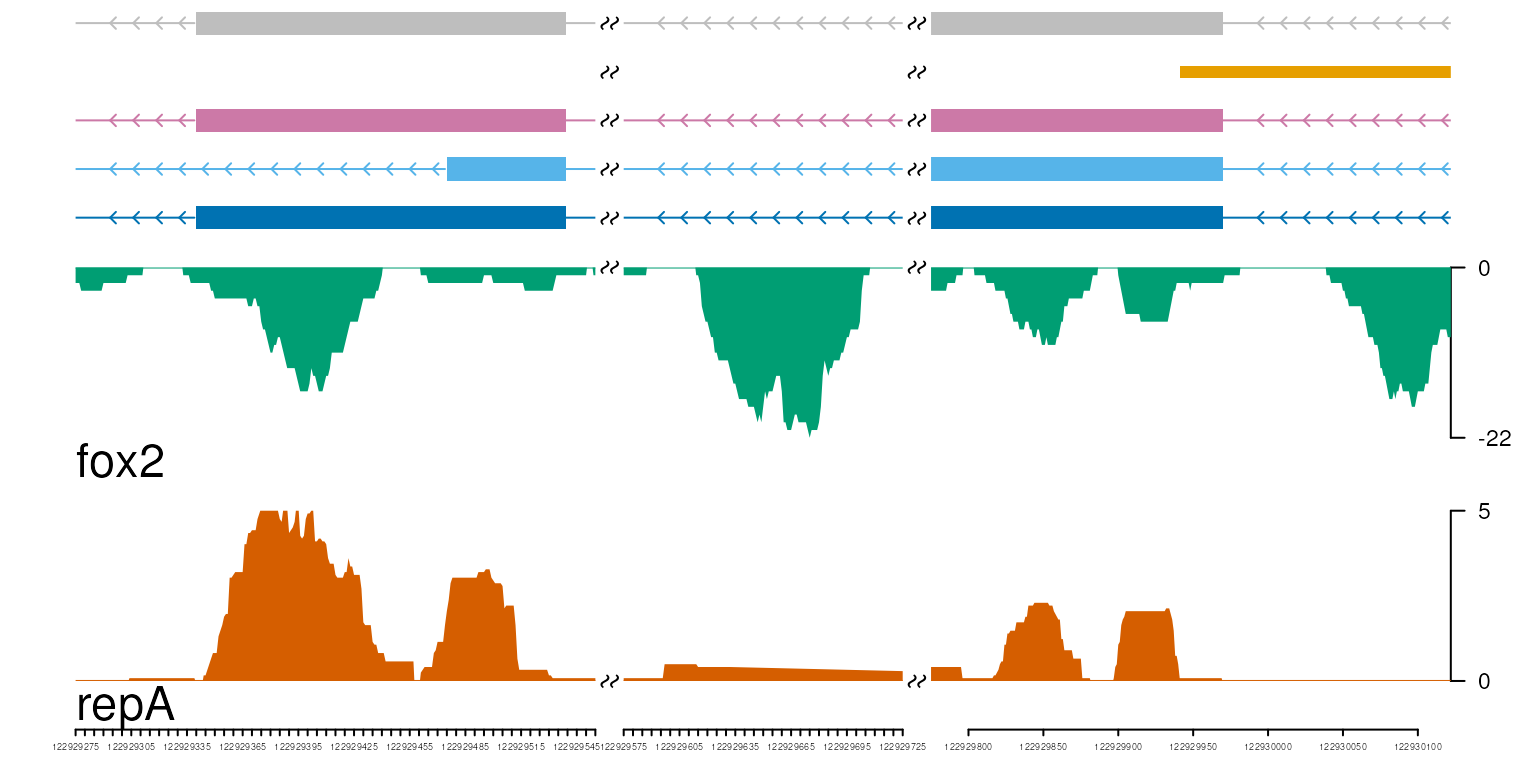

axis with breaks

Session Info

sessionInfo()

R version 4.4.1 (2024-06-14) Platform: x86_64-pc-linux-gnu Running under: Ubuntu 22.04.4 LTS

Matrix products: default BLAS: /usr/lib/x86_64-linux-gnu/openblas-pthread/libblas.so.3 LAPACK: /usr/lib/x86_64-linux-gnu/openblas-pthread/libopenblasp-r0.3.20.so; LAPACK version 3.10.0

locale: [1] LC_CTYPE=en_US.UTF-8 LC_NUMERIC=C
[3] LC_TIME=en_US.UTF-8 LC_COLLATE=en_US.UTF-8
[5] LC_MONETARY=en_US.UTF-8 LC_MESSAGES=en_US.UTF-8
[7] LC_PAPER=en_US.UTF-8 LC_NAME=C
[9] LC_ADDRESS=C LC_TELEPHONE=C
[11] LC_MEASUREMENT=en_US.UTF-8 LC_IDENTIFICATION=C

time zone: Etc/UTC tzcode source: system (glibc)

attached base packages: [1] grid stats4 stats graphics grDevices utils datasets [8] methods base

other attached packages: [1] httr_1.4.7
[2] VariantAnnotation_1.51.0
[3] Rsamtools_2.21.1
[4] Biostrings_2.73.1
[5] XVector_0.45.0
[6] SummarizedExperiment_1.35.1
[7] MatrixGenerics_1.17.0
[8] matrixStats_1.4.0
[9] org.Hs.eg.db_3.19.1
[10] TxDb.Hsapiens.UCSC.hg19.knownGene_3.2.2 [11] GenomicFeatures_1.57.0
[12] AnnotationDbi_1.67.0
[13] Biobase_2.65.1
[14] Gviz_1.49.0
[15] rtracklayer_1.65.0
[16] trackViewer_1.41.6
[17] GenomicRanges_1.57.1
[18] GenomeInfoDb_1.41.1
[19] IRanges_2.39.2
[20] S4Vectors_0.43.2
[21] BiocGenerics_0.51.1

loaded via a namespace (and not attached): [1] strawr_0.0.92 RColorBrewer_1.1-3 rstudioapi_0.16.0
[4] jsonlite_1.8.8 magrittr_2.0.3 rmarkdown_2.28
[7] fs_1.6.4 BiocIO_1.15.2 zlibbioc_1.51.1
[10] ragg_1.3.2 vctrs_0.6.5 memoise_2.0.1
[13] RCurl_1.98-1.16 base64enc_0.1-3 htmltools_0.5.8.1
[16] S4Arrays_1.5.7 progress_1.2.3 curl_5.2.2
[19] Rhdf5lib_1.27.0 rhdf5_2.49.0 SparseArray_1.5.31
[22] Formula_1.2-5 sass_0.4.9 bslib_0.8.0
[25] htmlwidgets_1.6.4 desc_1.4.3 httr2_1.0.3
[28] cachem_1.1.0 GenomicAlignments_1.41.0 lifecycle_1.0.4
[31] pkgconfig_2.0.3 Matrix_1.7-0 R6_2.5.1
[34] fastmap_1.2.0 GenomeInfoDbData_1.2.12 digest_0.6.37
[37] colorspace_2.1-1 textshaping_0.4.0 Hmisc_5.1-3
[40] RSQLite_2.3.7 filelock_1.0.3 fansi_1.0.6
[43] abind_1.4-5 compiler_4.4.1 bit64_4.0.5
[46] htmlTable_2.4.3 backports_1.5.0 BiocParallel_1.39.0
[49] DBI_1.2.3 highr_0.11 biomaRt_2.61.3
[52] rappdirs_0.3.3 DelayedArray_0.31.11 rjson_0.2.22
[55] tools_4.4.1 foreign_0.8-87 nnet_7.3-19
[58] glue_1.7.0 InteractionSet_1.33.0 restfulr_0.0.15
[61] rhdf5filters_1.17.0 checkmate_2.3.2 cluster_2.1.6
[64] generics_0.1.3 gtable_0.3.5 BSgenome_1.73.0
[67] ensembldb_2.29.1 data.table_1.16.0 hms_1.1.3
[70] xml2_1.3.6 utf8_1.2.4 pillar_1.9.0
[73] stringr_1.5.1 dplyr_1.1.4 BiocFileCache_2.13.0
[76] lattice_0.22-6 deldir_2.0-4 bit_4.0.5
[79] biovizBase_1.53.0 tidyselect_1.2.1 knitr_1.48
[82] gridExtra_2.3 ProtGenerics_1.37.1 xfun_0.47
[85] stringi_1.8.4 UCSC.utils_1.1.0 lazyeval_0.2.2
[88] yaml_2.3.10 evaluate_0.24.0 codetools_0.2-20
[91] interp_1.1-6 tibble_3.2.1 BiocManager_1.30.25
[94] cli_3.6.3 rpart_4.1.23 systemfonts_1.1.0
[97] munsell_0.5.1 jquerylib_0.1.4 Rcpp_1.0.13
[100] dichromat_2.0-0.1 grImport_0.9-7 dbplyr_2.5.0
[103] png_0.1-8 XML_3.99-0.17 parallel_4.4.1
[106] pkgdown_2.1.0 ggplot2_3.5.1 blob_1.2.4
[109] prettyunits_1.2.0 latticeExtra_0.6-30 jpeg_0.1-10
[112] AnnotationFilter_1.29.0 bitops_1.0-8 txdbmaker_1.1.1
[115] scales_1.3.0 crayon_1.5.3 BiocStyle_2.33.1
[118] rlang_1.1.4 KEGGREST_1.45.1

Jianhong Ou, Lihua Julie Zhu

5 September 2024

Prepare toy data

Using the `browseTracks` function as a helper

Adjust the x-axis or the X scale

Adjust the y-axis

Adjust the label of y-axis

Adjust the track color

Adjust the track height

Change the track names

Show paired data in the same track

Flip the x-axis

Optimize the theme

Plot with breaks

Session Info

trackViewer Vignette: change the track styles

Jianhong Ou, Lihua Julie Zhu

5 September 2024

Prepare toy data

Using the browseTracks function as a helper

Adjust the x-axis or the X scale

Adjust the y-axis

Adjust the label of y-axis

Adjust the track color

Adjust the track height

Change the track names

Show paired data in the same track

Flip the x-axis

Optimize the theme

Plot with breaks

Session Info

Using the `browseTracks` function as a helper